Introduction to SAS Essentials Mastering SAS for Data

Introduction to SAS Essentials Mastering SAS for Data Analytics Alan Elliott and Wayne Woodward 1 SAS ESSENTIALS -- Elliott & Woodward

Chapter 12: CORRELATION AND REGRESSION 2 SAS ESSENTIALS -- Elliott & Woodward

LEARNING OBJECTIVES • To be able to use SAS® procedures to calculate Pearson and Spearman correlations • To be able to use SAS procedures to produce a matrix of scatterplots • To be able to use SAS procedures to perform simple linear regression • To be able to use SAS procedures to perform multiple linear regression • To be able to use SAS procedures to calculate predictions using a model • To be able to use SAS procedures to perform residual analysis 3 SAS ESSENTIALS -- Elliott & Woodward

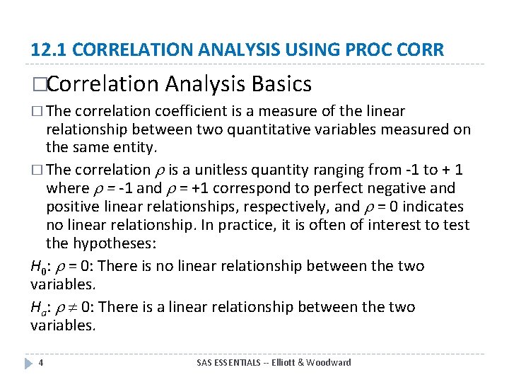
12. 1 CORRELATION ANALYSIS USING PROC CORR �Correlation Analysis Basics � The correlation coefficient is a measure of the linear relationship between two quantitative variables measured on the same entity. � The correlation is a unitless quantity ranging from -1 to + 1 where = -1 and = +1 correspond to perfect negative and positive linear relationships, respectively, and = 0 indicates no linear relationship. In practice, it is often of interest to test the hypotheses: H 0: = 0: There is no linear relationship between the two variables. Ha: 0: There is a linear relationship between the two variables. 4 SAS ESSENTIALS -- Elliott & Woodward

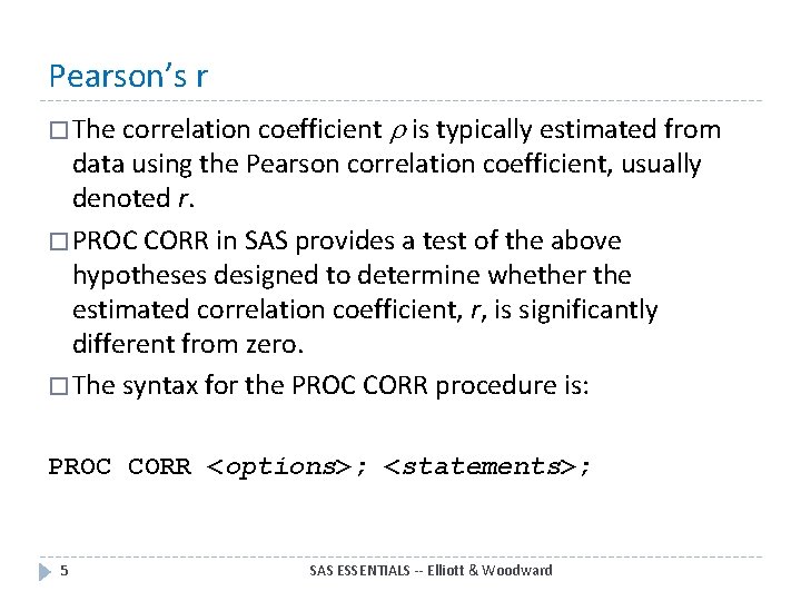
Pearson’s r � The correlation coefficient is typically estimated from data using the Pearson correlation coefficient, usually denoted r. � PROC CORR in SAS provides a test of the above hypotheses designed to determine whether the estimated correlation coefficient, r, is significantly different from zero. � The syntax for the PROC CORR procedure is: PROC CORR <options>; <statements>; 5 SAS ESSENTIALS -- Elliott & Woodward

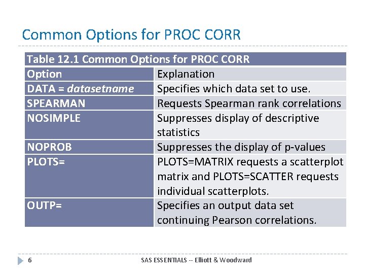
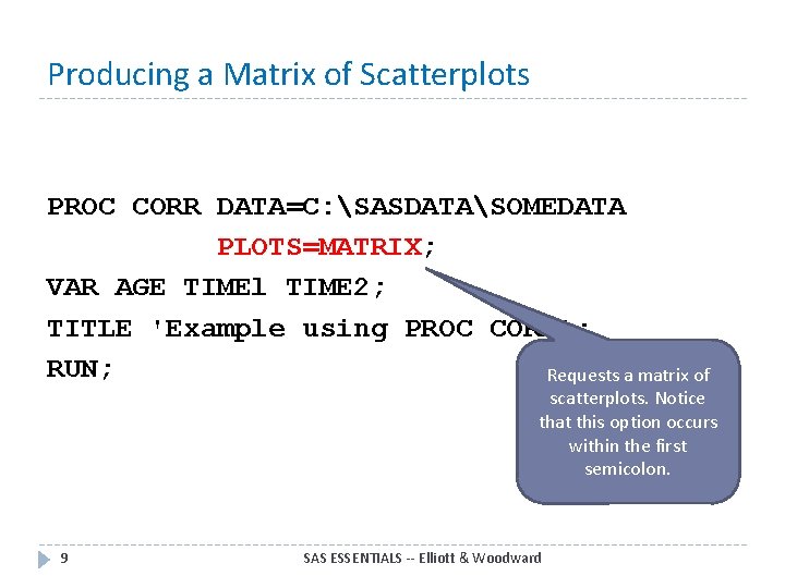
Common Options for PROC CORR Table 12. 1 Common Options for PROC CORR Option Explanation DATA = datasetname Specifies which data set to use. SPEARMAN Requests Spearman rank correlations NOSIMPLE Suppresses display of descriptive statistics NOPROB Suppresses the display of p-values PLOTS=MATRIX requests a scatterplot matrix and PLOTS=SCATTER requests individual scatterplots. OUTP= Specifies an output data set continuing Pearson correlations. 6 SAS ESSENTIALS -- Elliott & Woodward

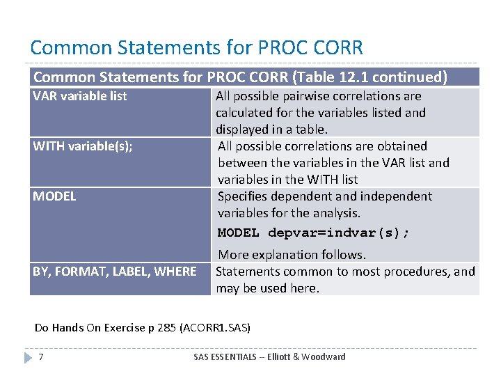
Common Statements for PROC CORR (Table 12. 1 continued) VAR variable list All possible pairwise correlations are calculated for the variables listed and displayed in a table. All possible correlations are obtained between the variables in the VAR list and variables in the WITH list Specifies dependent and independent variables for the analysis. MODEL depvar=indvar(s); WITH variable(s); MODEL BY, FORMAT, LABEL, WHERE More explanation follows. Statements common to most procedures, and may be used here. Do Hands On Exercise p 285 (ACORR 1. SAS) 7 SAS ESSENTIALS -- Elliott & Woodward

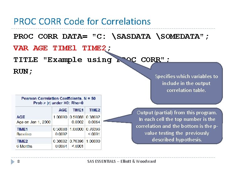
PROC CORR Code for Correlations PROC CORR DATA= "C: SASDATA SOMEDATA"; VAR AGE TIMEl TIME 2; TITLE "Example using PROC CORR"; RUN; Specifies which variables to include in the output correlation table. Output (partial) from this program. In each cell the top number is the correlation and the bottom is the pvalue testing the previously described hypothesis. 8 SAS ESSENTIALS -- Elliott & Woodward

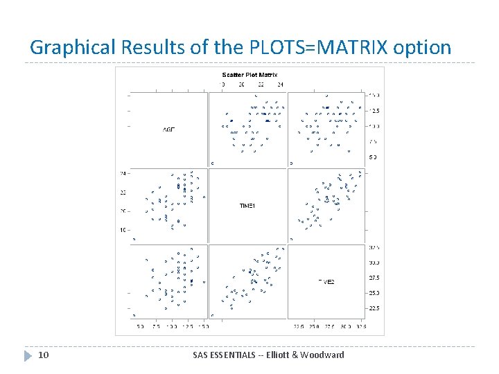
Producing a Matrix of Scatterplots PROC CORR DATA=C: SASDATASOMEDATA PLOTS=MATRIX; VAR AGE TIMEl TIME 2; TITLE 'Example using PROC CORR'; RUN; Requests a matrix of scatterplots. Notice that this option occurs within the first semicolon. 9 SAS ESSENTIALS -- Elliott & Woodward

Graphical Results of the PLOTS=MATRIX option 10 SAS ESSENTIALS -- Elliott & Woodward

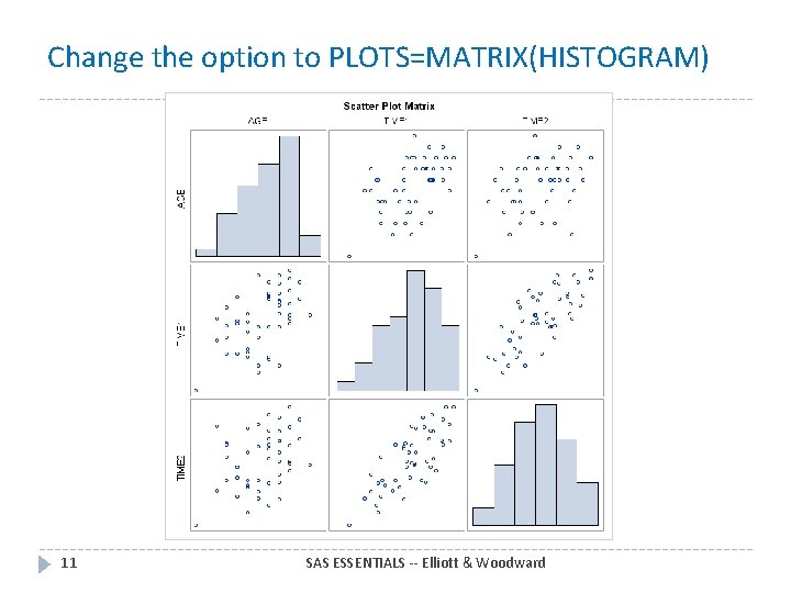
Change the option to PLOTS=MATRIX(HISTOGRAM) 11 SAS ESSENTIALS -- Elliott & Woodward

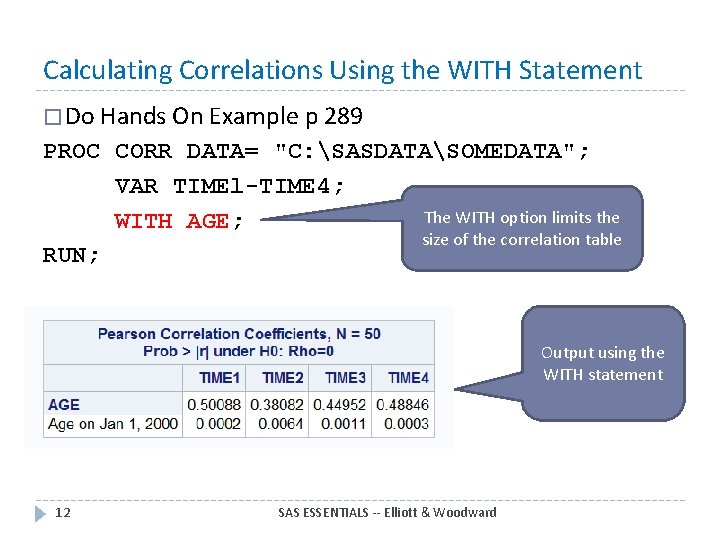
Calculating Correlations Using the WITH Statement � Do Hands On Example p 289 PROC CORR DATA= "C: SASDATASOMEDATA"; VAR TIMEl-TIME 4; The WITH option limits the WITH AGE; size of the correlation table RUN; Output using the WITH statement 12 SAS ESSENTIALS -- Elliott & Woodward

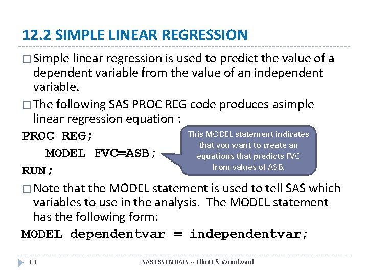
12. 2 SIMPLE LINEAR REGRESSION � Simple linear regression is used to predict the value of a dependent variable from the value of an independent variable. � The following SAS PROC REG code produces asimple linear regression equation : This MODEL statement indicates PROC REG; that you want to create an MODEL FVC=ASB; equations that predicts FVC from values of ASB. RUN; � Note that the MODEL statement is used to tell SAS which variables to use in the analysis. The MODEL statement has the following form: MODEL dependentvar = independentvar; 13 SAS ESSENTIALS -- Elliott & Woodward

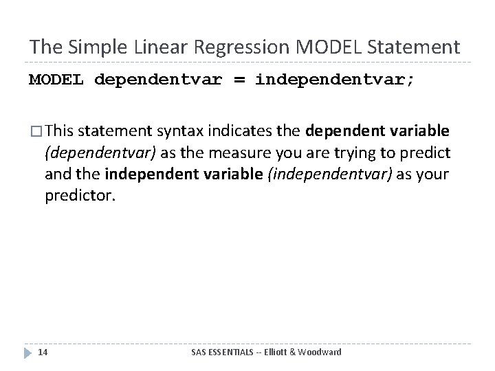
The Simple Linear Regression MODEL Statement MODEL dependentvar = independentvar; � This statement syntax indicates the dependent variable (dependentvar) as the measure you are trying to predict and the independent variable (independentvar) as your predictor. 14 SAS ESSENTIALS -- Elliott & Woodward

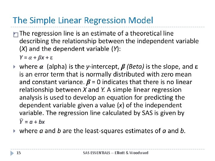
The Simple Linear Regression Model � 15 SAS ESSENTIALS -- Elliott & Woodward

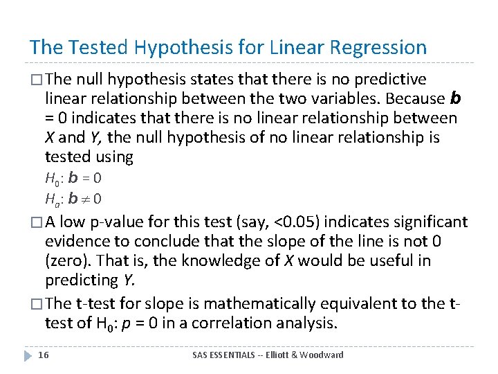
The Tested Hypothesis for Linear Regression � The null hypothesis states that there is no predictive linear relationship between the two variables. Because b = 0 indicates that there is no linear relationship between X and Y, the null hypothesis of no linear relationship is tested using H 0 : b = 0 Ha : b 0 � A low p-value for this test (say, <0. 05) indicates significant evidence to conclude that the slope of the line is not 0 (zero). That is, the knowledge of X would be useful in predicting Y. � The t-test for slope is mathematically equivalent to the ttest of H 0: p = 0 in a correlation analysis. 16 SAS ESSENTIALS -- Elliott & Woodward

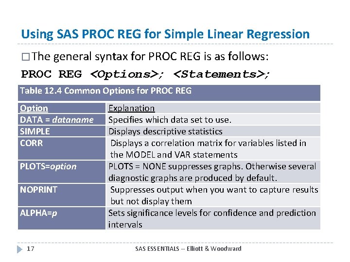
Using SAS PROC REG for Simple Linear Regression � The general syntax for PROC REG is as follows: PROC REG <Options>; <Statements>; Table 12. 4 Common Options for PROC REG Option DATA = dataname SIMPLE CORR PLOTS=option NOPRINT ALPHA=p 17 Explanation Specifies which data set to use. Displays descriptive statistics Displays a correlation matrix for variables listed in the MODEL and VAR statements PLOTS = NONE suppresses graphs. Otherwise several diagnostic graphs are produced by default. Suppresses output when you want to capture results but not display them Sets significance levels for confidence and prediction intervals SAS ESSENTIALS -- Elliott & Woodward

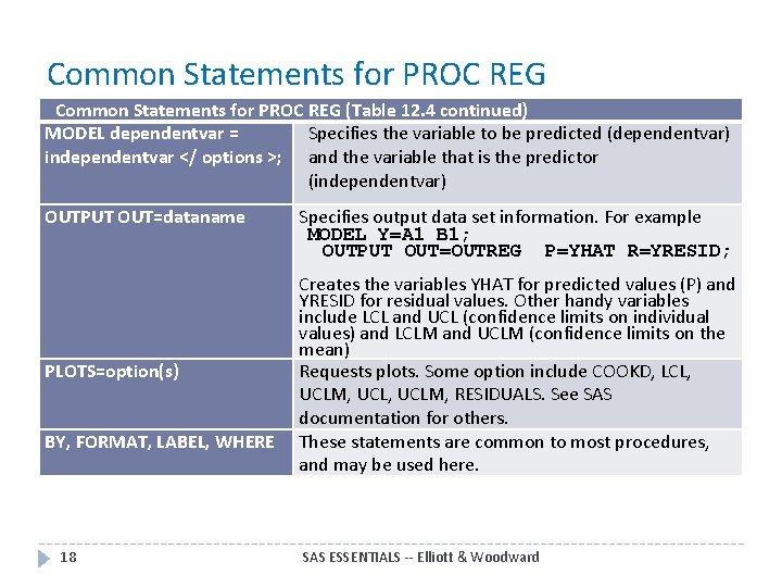
Common Statements for PROC REG (Table 12. 4 continued) MODEL dependentvar = Specifies the variable to be predicted (dependentvar) independentvar </ options >; and the variable that is the predictor (independentvar) OUTPUT OUT=dataname PLOTS=option(s) BY, FORMAT, LABEL, WHERE 18 Specifies output data set information. For example MODEL Y=A 1 B 1; OUTPUT OUT=OUTREG P=YHAT R=YRESID; Creates the variables YHAT for predicted values (P) and YRESID for residual values. Other handy variables include LCL and UCL (confidence limits on individual values) and LCLM and UCLM (confidence limits on the mean) Requests plots. Some option include COOKD, LCL, UCLM, RESIDUALS. See SAS documentation for others. These statements are common to most procedures, and may be used here. SAS ESSENTIALS -- Elliott & Woodward

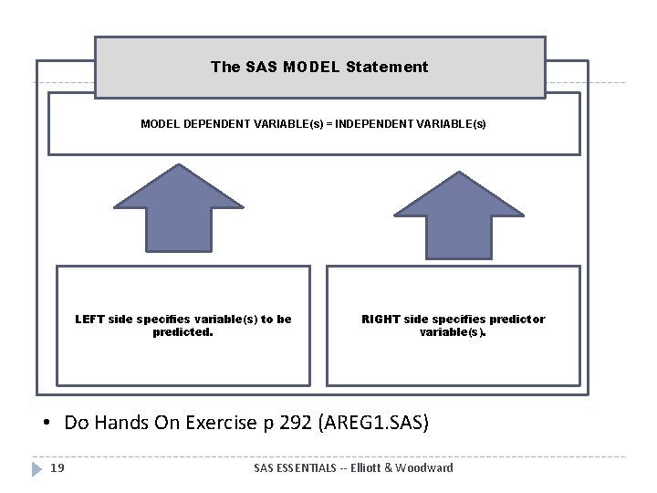
The SAS MODEL Statement MODEL DEPENDENT VARIABLE(s) = INDEPENDENT VARIABLE(s) LEFT side specifies variable(s) to be predicted. RIGHT side specifies predictor variable(s). • Do Hands On Exercise p 292 (AREG 1. SAS) 19 SAS ESSENTIALS -- Elliott & Woodward

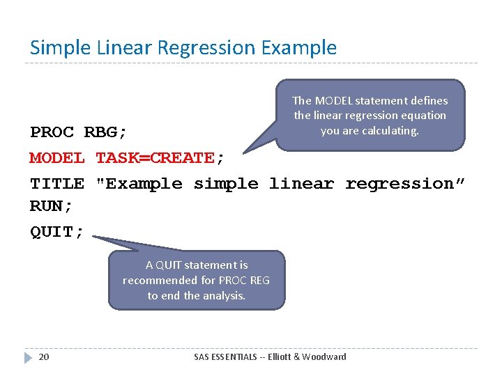
Simple Linear Regression Example The MODEL statement defines the linear regression equation you are calculating. PROC RBG; MODEL TASK=CREATE; TITLE "Example simple linear regression” RUN; QUIT; A QUIT statement is recommended for PROC REG to end the analysis. 20 SAS ESSENTIALS -- Elliott & Woodward

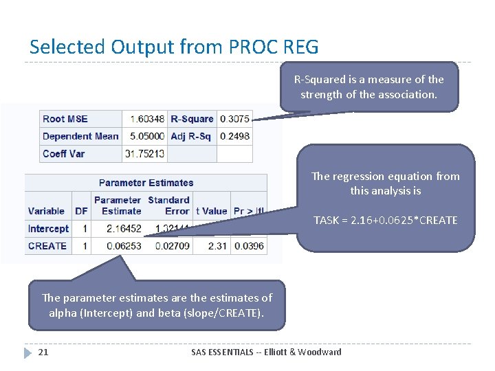
Selected Output from PROC REG R-Squared is a measure of the strength of the association. The regression equation from this analysis is TASK = 2. 16+0. 0625*CREATE The parameter estimates are the estimates of alpha (Intercept) and beta (slope/CREATE). 21 SAS ESSENTIALS -- Elliott & Woodward

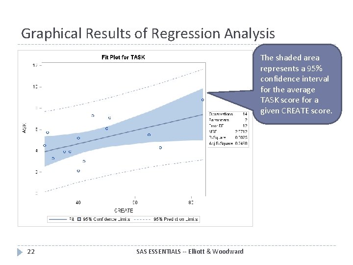
Graphical Results of Regression Analysis The shaded area represents a 95% confidence interval for the average TASK score for a given CREATE score. 22 SAS ESSENTIALS -- Elliott & Woodward

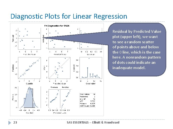
Diagnostic Plots for Linear Regression Residual by Predicted Value plot (upper left), we want to see a random scatter of points above and below the 0 line, which is the case here. A nonrandom pattern of dots could indicate an inadequate model. 23 SAS ESSENTIALS -- Elliott & Woodward

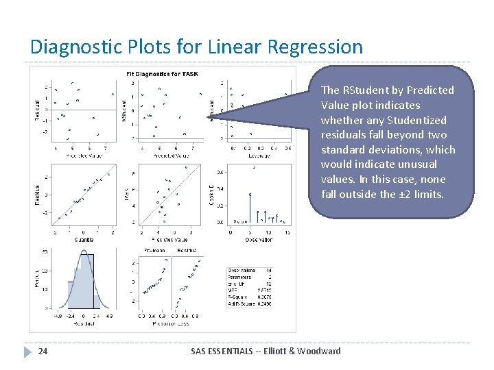
Diagnostic Plots for Linear Regression The RStudent by Predicted Value plot indicates whether any Studentized residuals fall beyond two standard deviations, which would indicate unusual values. In this case, none fall outside the ± 2 limits. 24 SAS ESSENTIALS -- Elliott & Woodward

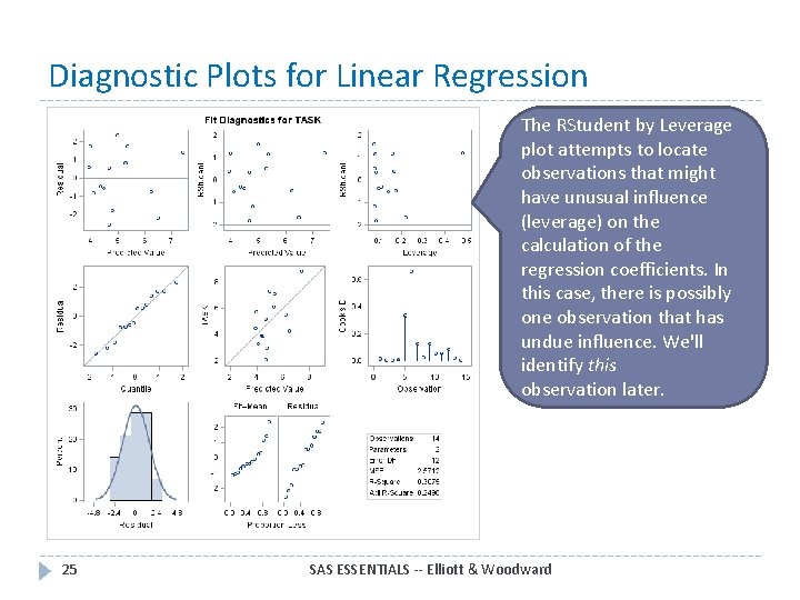
Diagnostic Plots for Linear Regression The RStudent by Leverage plot attempts to locate observations that might have unusual influence (leverage) on the calculation of the regression coefficients. In this case, there is possibly one observation that has undue influence. We'll identify this observation later. 25 SAS ESSENTIALS -- Elliott & Woodward

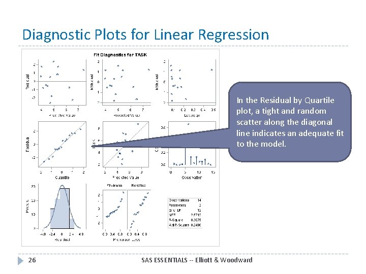
Diagnostic Plots for Linear Regression In the Residual by Quartile plot, a tight and random scatter along the diagonal line indicates an adequate fit to the model. 26 SAS ESSENTIALS -- Elliott & Woodward

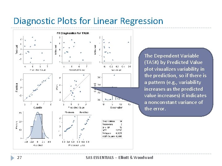
Diagnostic Plots for Linear Regression The Dependent Variable (TASK) by Predicted Value plot visualizes variability in the prediction, so if there is a pattern (e. g. , variability increases as the predicted value increases) it indicates a nonconstant variance of the error. 27 SAS ESSENTIALS -- Elliott & Woodward

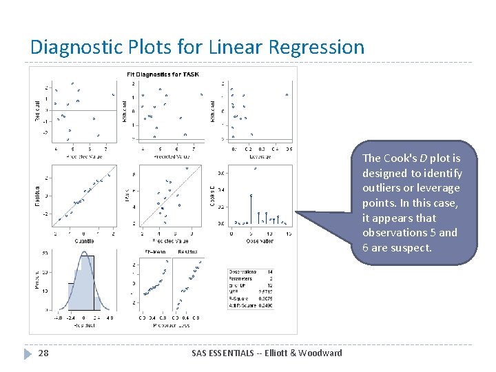
Diagnostic Plots for Linear Regression The Cook's D plot is designed to identify outliers or leverage points. In this case, it appears that observations 5 and 6 are suspect. 28 SAS ESSENTIALS -- Elliott & Woodward

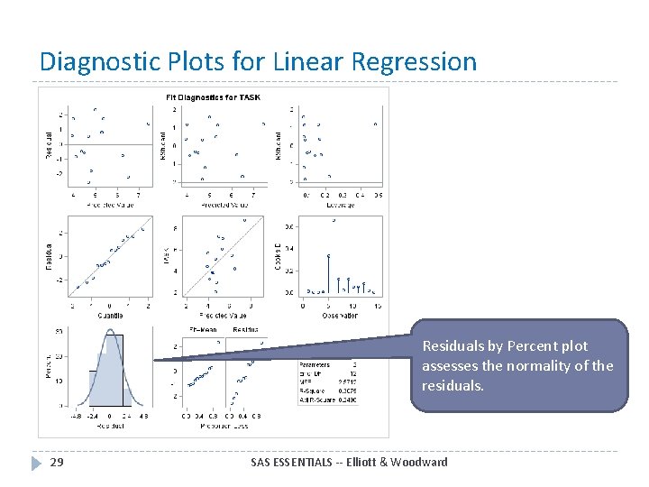
Diagnostic Plots for Linear Regression Residuals by Percent plot assesses the normality of the residuals. 29 SAS ESSENTIALS -- Elliott & Woodward

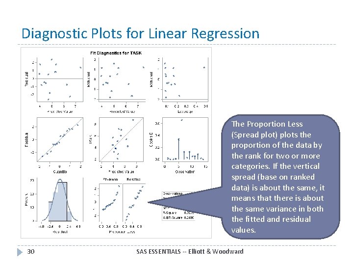
Diagnostic Plots for Linear Regression The Proportion Less (Spread plot) plots the proportion of the data by the rank for two or more categories. If the vertical spread (base on ranked data) is about the same, it means that there is about the same variance in both the fitted and residual values. 30 SAS ESSENTIALS -- Elliott & Woodward

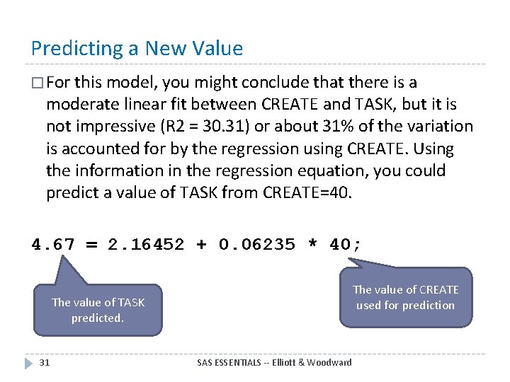
Predicting a New Value � For this model, you might conclude that there is a moderate linear fit between CREATE and TASK, but it is not impressive (R 2 = 30. 31) or about 31% of the variation is accounted for by the regression using CREATE. Using the information in the regression equation, you could predict a value of TASK from CREATE=40. 4. 67 = 2. 16452 + 0. 06235 * 40; The value of CREATE used for prediction The value of TASK predicted. 31 SAS ESSENTIALS -- Elliott & Woodward

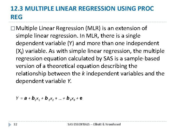
12. 3 MULTIPLE LINEAR REGRESSION USING PROC REG � Multiple Linear Regression (MLR) is an extension of simple linear regression. In MLR, there is a single dependent variable (Y) and more than one independent (Xi) variable. As with simple linear regression, the multiple regression equation calculated by SAS is a sample-based version of a theoretical equation describing the relationship between the k independent variables and the dependent variable Y. Y = a + b 1 x 1 + b 2 x 2 + … + b k xk + e 32 SAS ESSENTIALS -- Elliott & Woodward

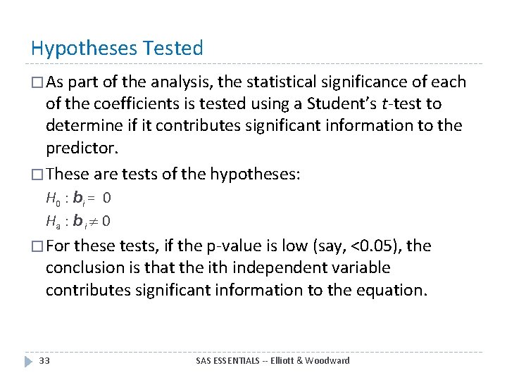
Hypotheses Tested � As part of the analysis, the statistical significance of each of the coefficients is tested using a Student’s t-test to determine if it contributes significant information to the predictor. � These are tests of the hypotheses: H 0 : b i = 0 Ha : b i 0 � For these tests, if the p-value is low (say, <0. 05), the conclusion is that the ith independent variable contributes significant information to the equation. 33 SAS ESSENTIALS -- Elliott & Woodward

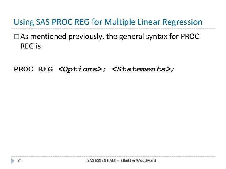
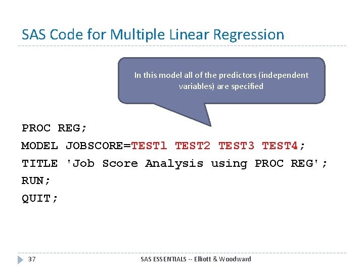
Using SAS PROC REG for Multiple Linear Regression � As mentioned previously, the REG is general syntax for PROC REG <Options>; <Statements>; 34 SAS ESSENTIALS -- Elliott & Woodward

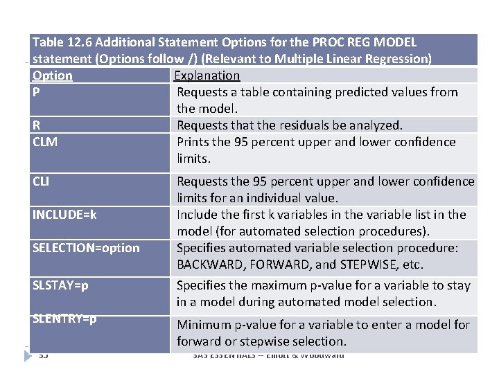
Table 12. 6 Additional Statement Options for the PROC REG MODEL statement (Options follow /) (Relevant to Multiple Linear Regression) Option Explanation P Requests a table containing predicted values from the model. R Requests that the residuals be analyzed. CLM Prints the 95 percent upper and lower confidence limits. CLI INCLUDE=k SELECTION=option SLSTAY=p SLENTRY=p 35 Requests the 95 percent upper and lower confidence limits for an individual value. Include the first k variables in the variable list in the model (for automated selection procedures). Specifies automated variable selection procedure: BACKWARD, FORWARD, and STEPWISE, etc. Specifies the maximum p-value for a variable to stay in a model during automated model selection. Minimum p-value for a variable to enter a model forward or stepwise selection. SAS ESSENTIALS -- Elliott & Woodward

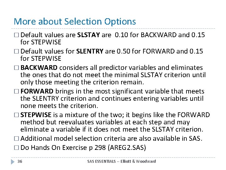
More about Selection Options � Default values are SLSTAY are 0. 10 for BACKWARD and 0. 15 for STEPWISE � Default values for SLENTRY are 0. 50 for FORWARD and 0. 15 for STEPWISE � BACKWARD considers all predictor variables and eliminates the ones that do not meet the minimal SLSTAY criterion until only those meeting the criterion remain. � FORWARD brings in the most significant variable that meets the SLENTRY criterion and continues entering variables until none meets the criterion. � STEPWISE is a mixture of the two; it begins like the FORWARD method but reevaluates variables at each step and may eliminate a variable if it does not meet the SLSTAY criterion. � Additional model selection criteria are also available in SAS. � Do Hands On Exercise p 298 (AREG 2. SAS) 36 SAS ESSENTIALS -- Elliott & Woodward

SAS Code for Multiple Linear Regression In this model all of the predictors (independent variables) are specified PROC REG; MODEL JOBSCORE=TESTl TEST 2 TEST 3 TEST 4; TITLE 'Job Score Analysis using PROC REG'; RUN; QUIT; 37 SAS ESSENTIALS -- Elliott & Woodward

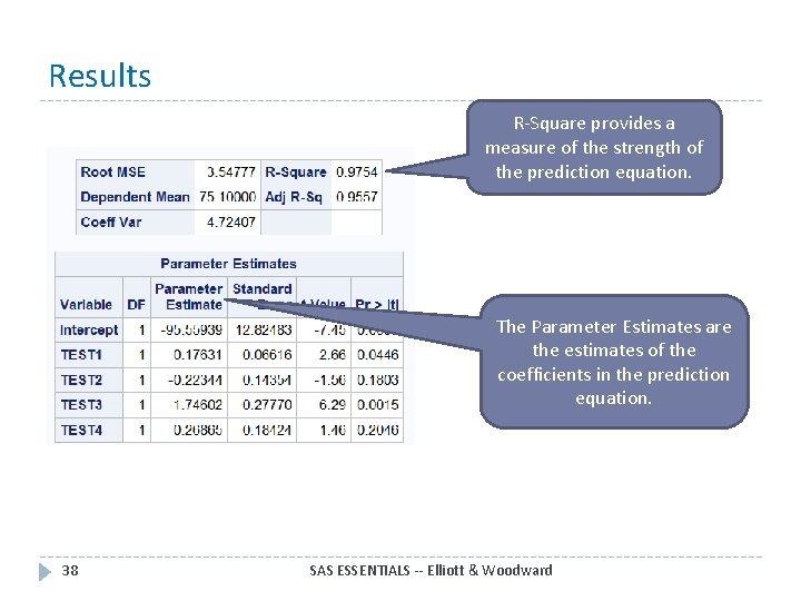
Results R-Square provides a measure of the strength of the prediction equation. The Parameter Estimates are the estimates of the coefficients in the prediction equation. 38 SAS ESSENTIALS -- Elliott & Woodward

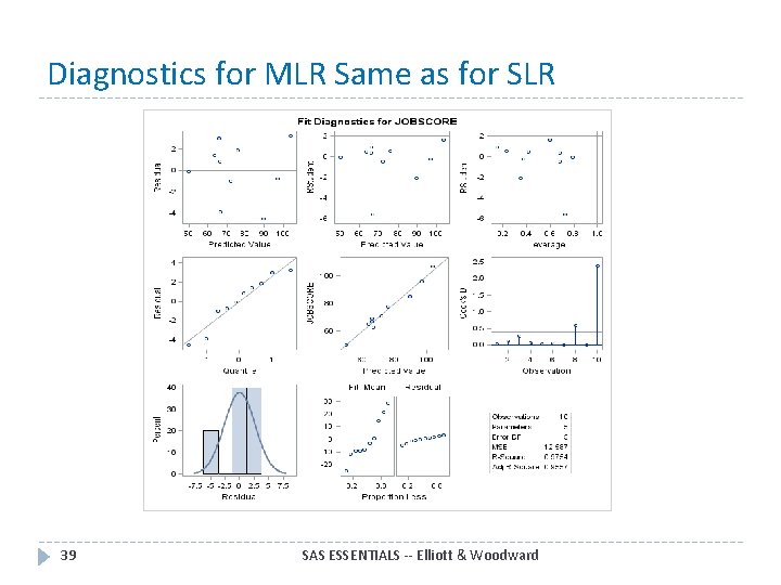
Diagnostics for MLR Same as for SLR 39 SAS ESSENTIALS -- Elliott & Woodward

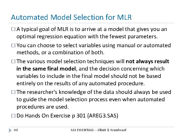
Automated Model Selection for MLR � A typical goal of MLR is to arrive at a model that gives you an optimal regression equation with the fewest parameters. � You can choose to select variables using manual or automated methods, or a combination of both. � The various model selection techniques will not always result in the same final model, and the decision concerning which variables to include in the final model should not be based entirely on the results of any automated procedure. � The researcher's knowledge of the data should always be used to guide the model selection process even when automated procedures are used. � Do Hands On Exercise p 301 (AREG 3. SAS) 40 SAS ESSENTIALS -- Elliott & Woodward

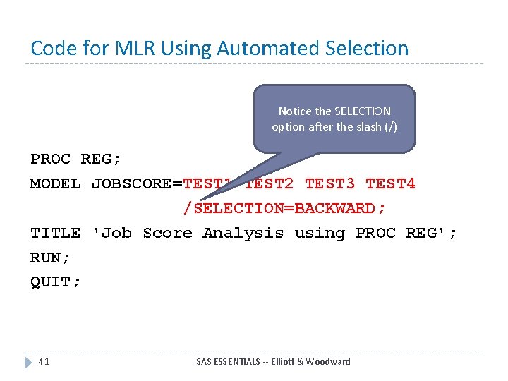
Code for MLR Using Automated Selection Notice the SELECTION option after the slash (/) PROC REG; MODEL JOBSCORE=TEST 1 TEST 2 TEST 3 TEST 4 /SELECTION=BACKWARD; TITLE 'Job Score Analysis using PROC REG'; RUN; QUIT; 41 SAS ESSENTIALS -- Elliott & Woodward

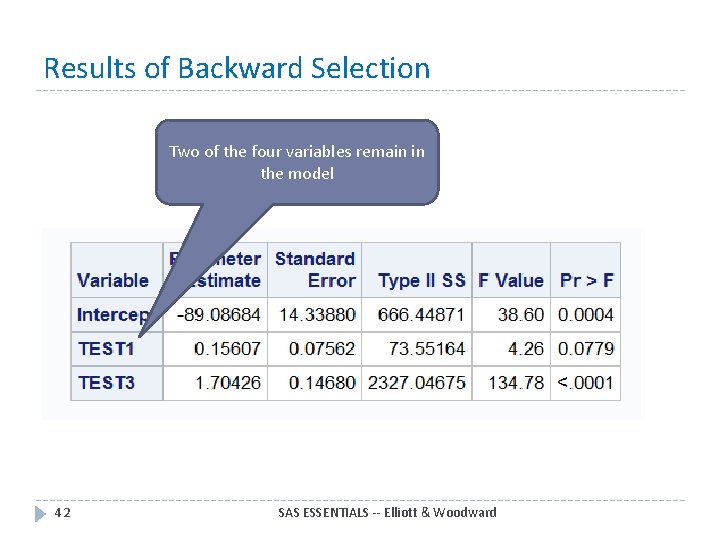
Results of Backward Selection Two of the four variables remain in the model 42 SAS ESSENTIALS -- Elliott & Woodward

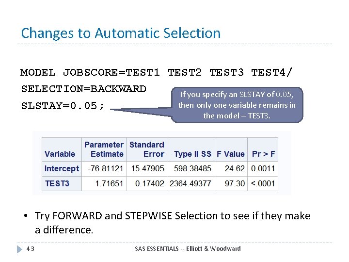
Changes to Automatic Selection MODEL JOBSCORE=TEST 1 TEST 2 TEST 3 TEST 4/ SELECTION=BACKWARD If you specify an SLSTAY of 0. 05, then only one variable remains in SLSTAY=0. 05; the model – TEST 3. • Try FORWARD and STEPWISE Selection to see if they make a difference. 43 SAS ESSENTIALS -- Elliott & Woodward

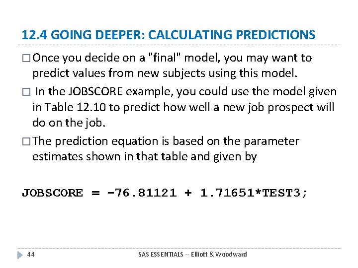
12. 4 GOING DEEPER: CALCULATING PREDICTIONS � Once you decide on a "final" model, you may want to predict values from new subjects using this model. � In the JOBSCORE example, you could use the model given in Table 12. 10 to predict how well a new job prospect will do on the job. � The prediction equation is based on the parameter estimates shown in that table and given by JOBSCORE = -76. 81121 + 1. 71651*TEST 3; 44 SAS ESSENTIALS -- Elliott & Woodward

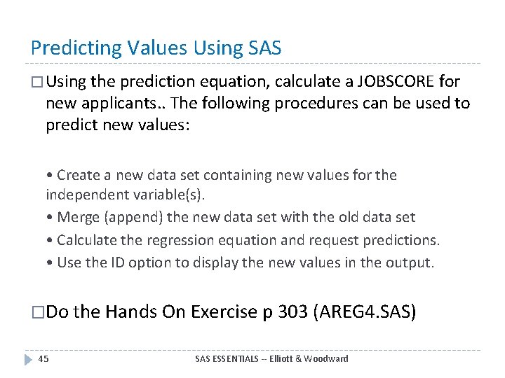
Predicting Values Using SAS � Using the prediction equation, calculate a JOBSCORE for new applicants. . The following procedures can be used to predict new values: • Create a new data set containing new values for the independent variable(s). • Merge (append) the new data set with the old data set • Calculate the regression equation and request predictions. • Use the ID option to display the new values in the output. �Do the Hands On Exercise p 303 (AREG 4. SAS) 45 SAS ESSENTIALS -- Elliott & Woodward

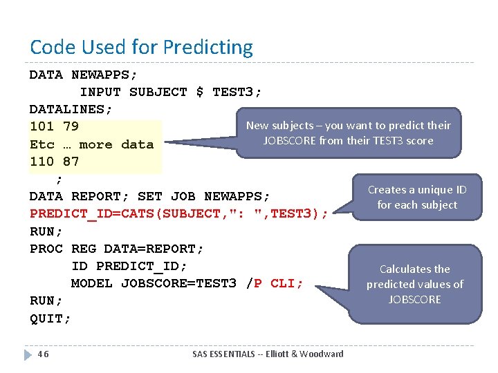
Code Used for Predicting DATA NEWAPPS; INPUT SUBJECT $ TEST 3; DATALINES; New subjects – you want to predict their 101 79 JOBSCORE from their TEST 3 score Etc … more data 110 87 ; Creates a unique ID DATA REPORT; SET JOB NEWAPPS; for each subject PREDICT_ID=CATS(SUBJECT, ": ", TEST 3); RUN; PROC REG DATA=REPORT; ID PREDICT_ID; Calculates the MODEL JOBSCORE=TEST 3 /P CLI; predicted values of JOBSCORE RUN; QUIT; 46 SAS ESSENTIALS -- Elliott & Woodward

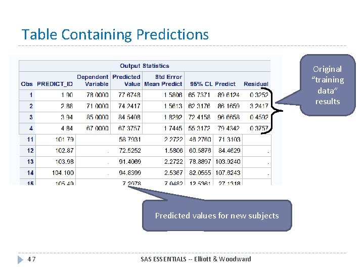
Table Containing Predictions Original “training data” results Predicted values for new subjects 47 SAS ESSENTIALS -- Elliott & Woodward

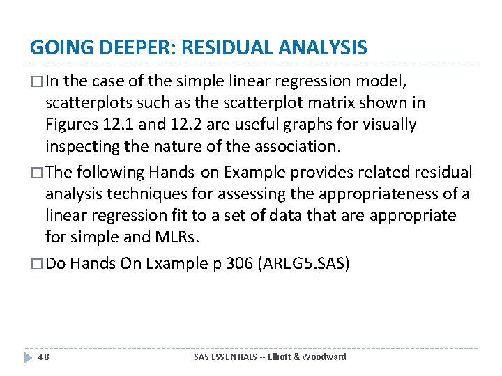
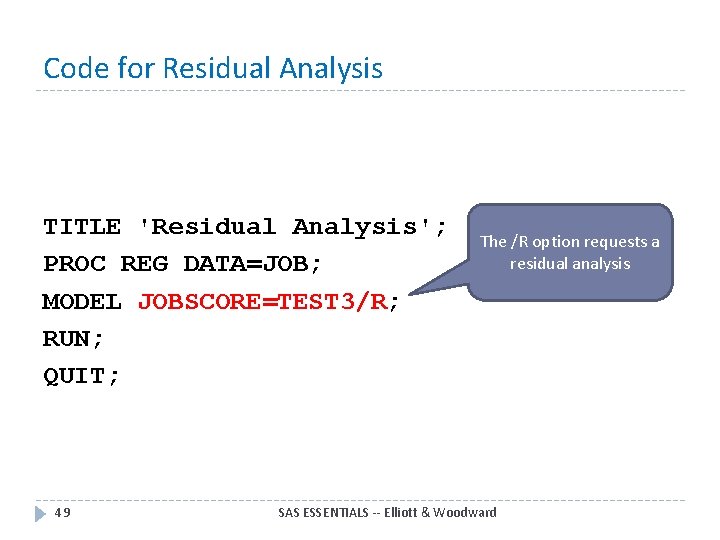
GOING DEEPER: RESIDUAL ANALYSIS � In the case of the simple linear regression model, scatterplots such as the scatterplot matrix shown in Figures 12. 1 and 12. 2 are useful graphs for visually inspecting the nature of the association. � The following Hands-on Example provides related residual analysis techniques for assessing the appropriateness of a linear regression fit to a set of data that are appropriate for simple and MLRs. � Do Hands On Example p 306 (AREG 5. SAS) 48 SAS ESSENTIALS -- Elliott & Woodward

Code for Residual Analysis TITLE 'Residual Analysis'; PROC REG DATA=JOB; MODEL JOBSCORE=TEST 3/R; RUN; QUIT; 49 The /R option requests a residual analysis SAS ESSENTIALS -- Elliott & Woodward

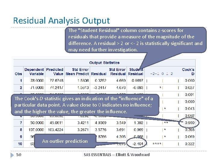
Residual Analysis Output The "Student Residual" column contains z-scores for residuals that provide a measure of the magnitude of the difference. A residual > 2 or <- 2 is statistically significant and may need further investigation. The Cook's D statistic gives an indication of the "influence" of a particular data point. A value close to 0 indicates no influence; and the higher the value, the greater the influence. An outlier prediction 50 SAS ESSENTIALS -- Elliott & Woodward

12. 6 SUMMARY � This chapter shows you how to measure the association between two quantitative variables (correlation analysis). It also discusses how to calculate a prediction equation using simple or multiple linear regression. � Continue to Chapter 13: 51 ANALYSIS OF VARIANCE SAS ESSENTIALS -- Elliott & Woodward

These slides are based on the book: Introduction to SAS Essentials Mastering SAS for Data Analytics, 2 nd Edition By Alan C, Elliott and Wayne A. Woodward Paperback: 512 pages Publisher: Wiley; 2 edition (August 3, 2015) Language: English ISBN-10: 111904216 X ISBN-13: 978 -1119042167 These slides are provided for you to use to teach SAS using this book. Feel free to modify them for your own needs. Please send comments about errors in the slides (or suggestions for improvements) to acelliott@smu. edu. Thanks. 52 SAS ESSENTIALS -- Elliott & Woodward