Introduction to Halide Sander Vocke 5 LIM 0

Introduction to Halide Sander Vocke – 5 LIM 0 – 17 -03 -2016

What? • Two guest lectures about the Halide language and compiler. Today, using a 3 x 3 Blur algorithm as leading example, we answer: • What is it? • How to use it? • Why to use it? Next time (March 31 st): • How does the Halide compiler work? 2

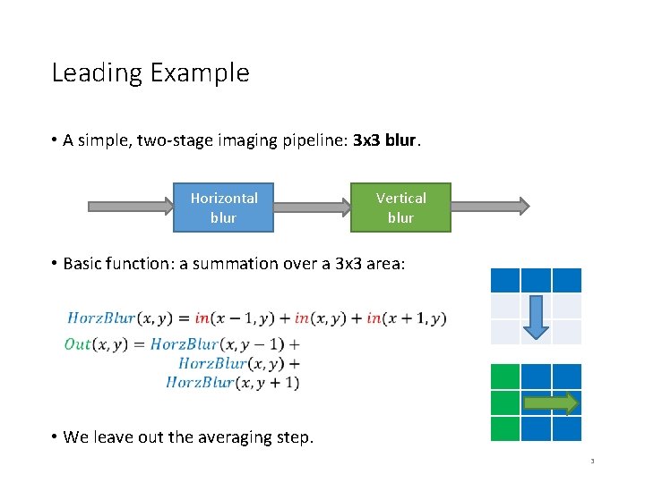
Leading Example • A simple, two-stage imaging pipeline: 3 x 3 blur. Horizontal blur Vertical blur • Basic function: a summation over a 3 x 3 area: • We leave out the averaging step. 3

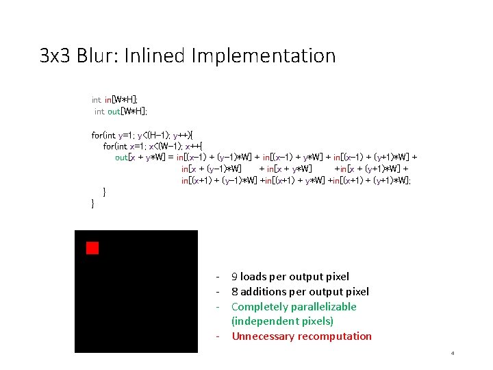
3 x 3 Blur: Inlined Implementation int in[W*H]; int out[W*H]; for(int y=1; y<(H-1); y++){ for(int x=1; x<(W-1); x++{ out[x + y*W] = in[(x-1) + (y-1)*W] + in[(x-1) + y*W] + in[(x-1) + (y+1)*W] + in[x + (y-1)*W] + in[x + y*W] +in[x + (y+1)*W] + in[(x+1) + (y-1)*W] +in[(x+1) + y*W] +in[(x+1) + (y+1)*W]; } } - 9 loads per output pixel - 8 additions per output pixel - Completely parallelizable (independent pixels) - Unnecessary recomputation 4

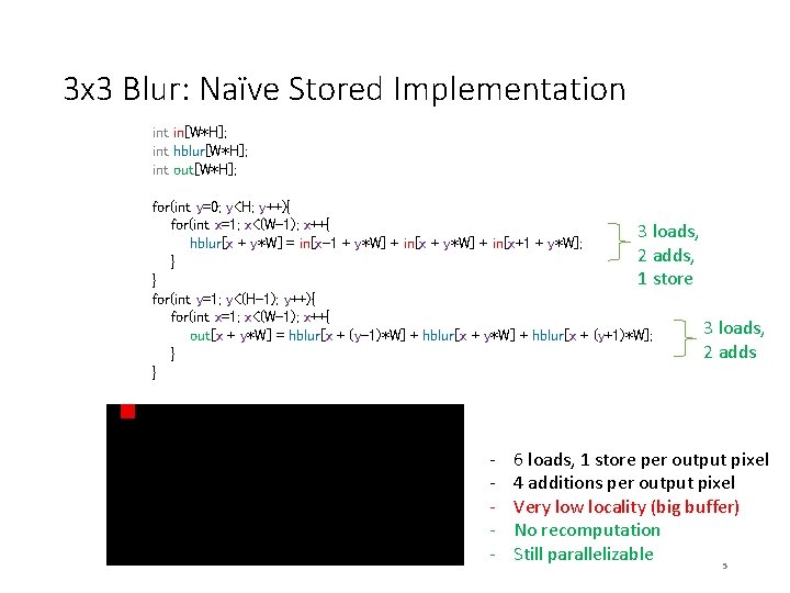
3 x 3 Blur: Naïve Stored Implementation int in[W*H]; int hblur[W*H]; int out[W*H]; for(int y=0; y<H; y++){ for(int x=1; x<(W-1); x++{ 3 loads, hblur[x + y*W] = in[x-1 + y*W] + in[x+1 + y*W]; 2 adds, } 1 store } for(int y=1; y<(H-1); y++){ for(int x=1; x<(W-1); x++{ 3 loads, out[x + y*W] = hblur[x + (y-1)*W] + hblur[x + y*W] + hblur[x + (y+1)*W]; 2 adds } } - 6 loads, 1 store per output pixel 4 additions per output pixel Very low locality (big buffer) No recomputation Still parallelizable 5

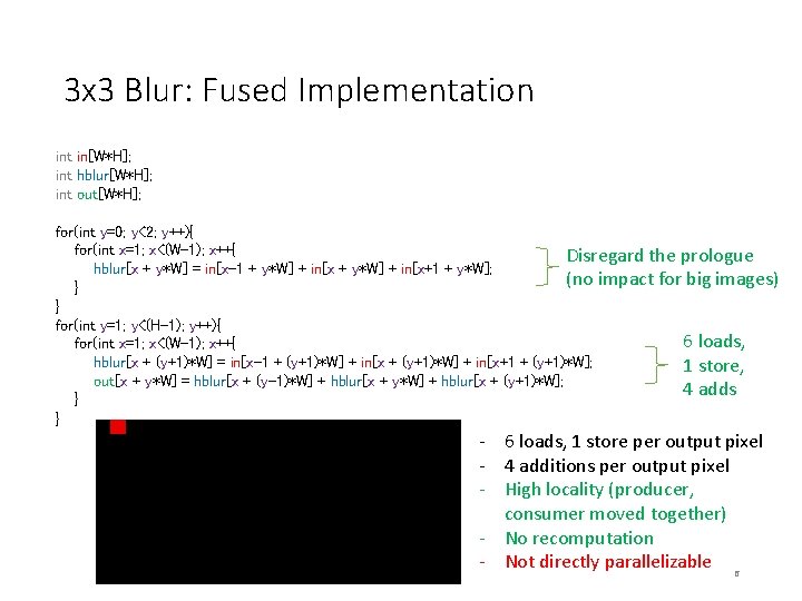
3 x 3 Blur: Fused Implementation int in[W*H]; int hblur[W*H]; int out[W*H]; for(int y=0; y<2; y++){ for(int x=1; x<(W-1); x++{ Disregard the prologue hblur[x + y*W] = in[x-1 + y*W] + in[x+1 + y*W]; (no impact for big images) } } for(int y=1; y<(H-1); y++){ 6 loads, for(int x=1; x<(W-1); x++{ hblur[x + (y+1)*W] = in[x-1 + (y+1)*W] + in[x+1 + (y+1)*W]; 1 store, out[x + y*W] = hblur[x + (y-1)*W] + hblur[x + y*W] + hblur[x + (y+1)*W]; 4 adds } } - 6 loads, 1 store per output pixel - 4 additions per output pixel - High locality (producer, consumer moved together) - No recomputation - Not directly parallelizable 6

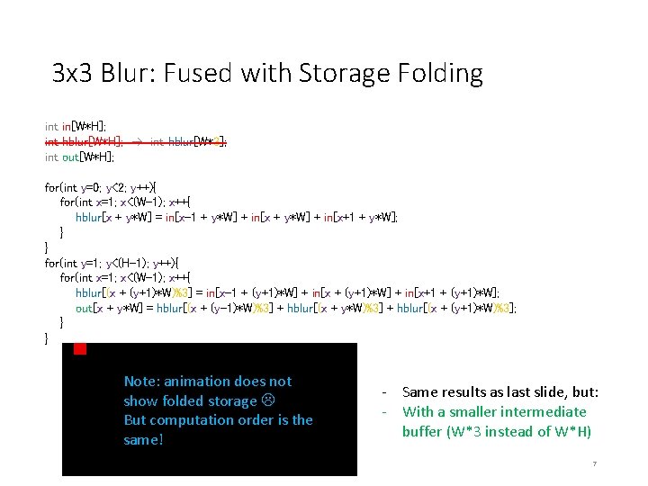
3 x 3 Blur: Fused with Storage Folding int in[W*H]; int hblur[W*H]; int hblur[W*3]; int out[W*H]; for(int y=0; y<2; y++){ for(int x=1; x<(W-1); x++{ hblur[x + y*W] = in[x-1 + y*W] + in[x+1 + y*W]; } } for(int y=1; y<(H-1); y++){ for(int x=1; x<(W-1); x++{ hblur[(x + (y+1)*W)%3] = in[x-1 + (y+1)*W] + in[x+1 + (y+1)*W]; out[x + y*W] = hblur[(x + (y-1)*W)%3] + hblur[(x + y*W)%3] + hblur[(x + (y+1)*W)%3]; } } Note: animation does not show folded storage But computation order is the same! - Same results as last slide, but: - With a smaller intermediate buffer (W*3 instead of W*H) 7

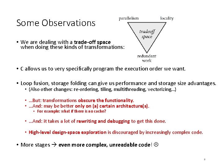
Some Observations • We are dealing with a trade-off space when doing these kinds of transformations: • C allows us to very specifically program the execution order we want. • Loop fusion, storage folding can give us performance and storage size advantages. • (Also other changes: re-ordering, tiling, multithreading, vectorizing…) • …But: transformations obscure the functionality. • …And: may be better only on (a) certain architecture(s). • For example: what if there is no cache? • …And: it takes a lot of rewriting and debugging to get this done. • High-level design-space exploration is discouraged by increasingly complex code. • More stages even more complex, unreadable code! 8

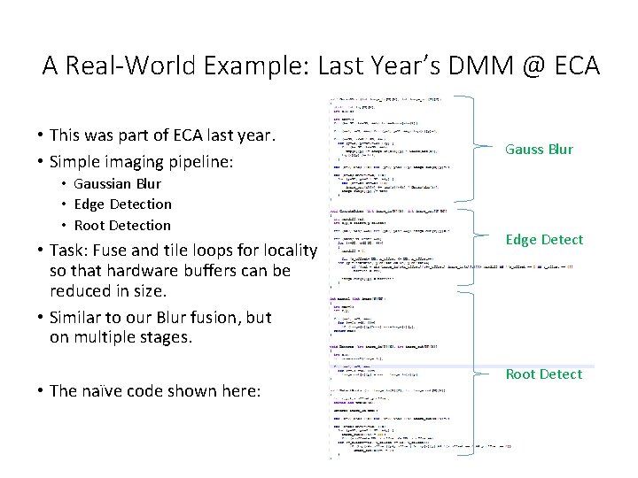
A Real-World Example: Last Year’s DMM @ ECA • This was part of ECA last year. • Simple imaging pipeline: • Gaussian Blur • Edge Detection • Root Detection • Task: Fuse and tile loops for locality so that hardware buffers can be reduced in size. • Similar to our Blur fusion, but on multiple stages. • The naïve code shown here: Gauss Blur Edge Detect Root Detect 9

A Real-World Example: Last Year’s DMM @ ECA • Fusing those loops together required some prior work: • Re-ordering nested loops to match the direction of computation • Each loop had different boundary conditions due to edge pixel dependencies • As many imaging algorithms do! • Leads to a multitude of nested pro- and epilogues when fusing. • Tiling makes the boundary condition problem even worse • Boundary conditions of tiles in image • Boundary conditions of pixels in tiles • So, what did the code look like after fusing? 10

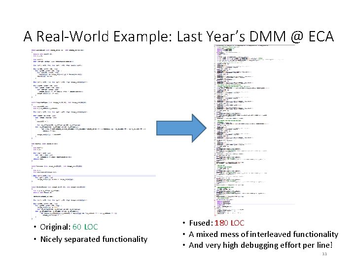
A Real-World Example: Last Year’s DMM @ ECA • Original: 60 LOC • Nicely separated functionality • Fused: 180 LOC • A mixed mess of interleaved functionality • And very high debugging effort per line! 11

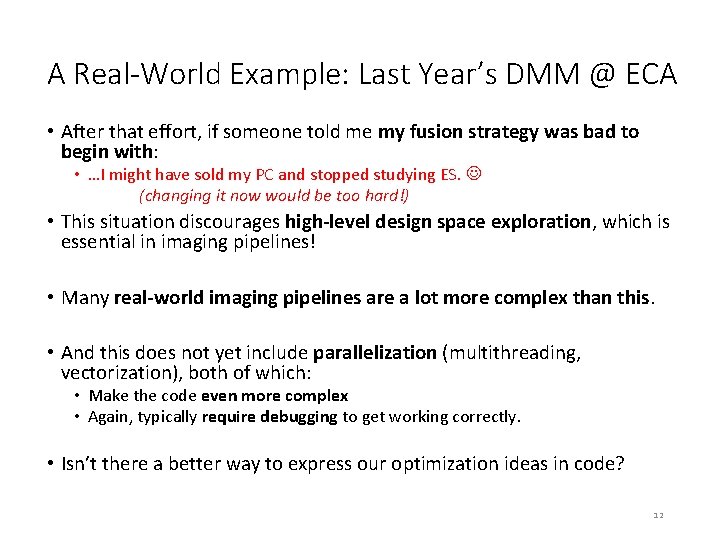
A Real-World Example: Last Year’s DMM @ ECA • After that effort, if someone told me my fusion strategy was bad to begin with: • …I might have sold my PC and stopped studying ES. (changing it now would be too hard!) • This situation discourages high-level design space exploration, which is essential in imaging pipelines! • Many real-world imaging pipelines are a lot more complex than this. • And this does not yet include parallelization (multithreading, vectorization), both of which: • Make the code even more complex • Again, typically require debugging to get working correctly. • Isn’t there a better way to express our optimization ideas in code? 12

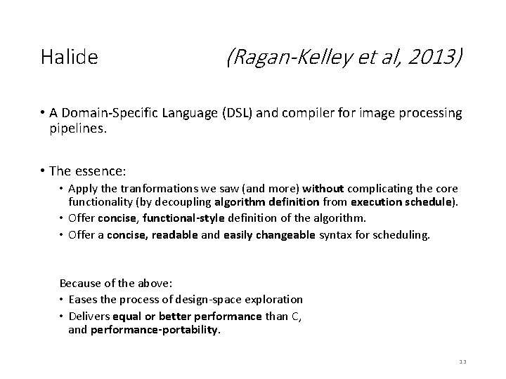
Halide (Ragan-Kelley et al, 2013) • A Domain-Specific Language (DSL) and compiler for image processing pipelines. • The essence: • Apply the tranformations we saw (and more) without complicating the core functionality (by decoupling algorithm definition from execution schedule). • Offer concise, functional-style definition of the algorithm. • Offer a concise, readable and easily changeable syntax for scheduling. Because of the above: • Eases the process of design-space exploration • Delivers equal or better performance than C, and performance-portability. 13

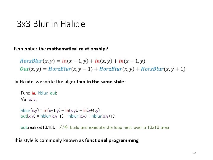
3 x 3 Blur in Halide Remember the mathematical relationship? In Halide, we write the algorithm in the same style: Func in, hblur, out; Var x, y; hblur(x, y) = in(x-1, y) + in(x, y), + in(x+1, y); out(x, y) = hblur(x, y-1) + hblur(x, y+1); out. realize(10, 10); // build and execute the loop nest over a 10 x 10 area This style is commonly known as functional programming. 14

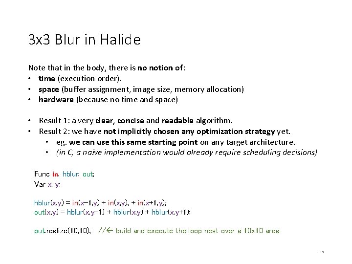
3 x 3 Blur in Halide Note that in the body, there is no notion of: • time (execution order). • space (buffer assignment, image size, memory allocation) • hardware (because no time and space) • Result 1: a very clear, concise and readable algorithm. • Result 2: we have not implicitly chosen any optimization strategy yet. • eg. we can use this same starting point on any target architecture. • (in C, a naïve implementation would already require scheduling decisions) Func in, hblur, out; Var x, y; hblur(x, y) = in(x-1, y) + in(x, y), + in(x+1, y); out(x, y) = hblur(x, y-1) + hblur(x, y+1); out. realize(10, 10); // build and execute the loop nest over a 10 x 10 area 15

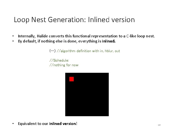
Loop Nest Generation: Inlined version • Internally, Halide converts this functional representation to a C-like loop nest. • By default, if nothing else is done, everything is inlined. (…) //algorithm definition with in, hblur, out //Schedule: //nothing for now • Equivalent to our inlined version! 16

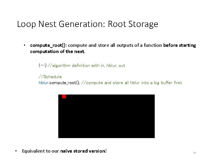
Loop Nest Generation: Root Storage • compute_root(): compute and store all outputs of a function before starting computation of the next. (…) //algorithm definition with in, hblur, out //Schedule: hblur. compute_root(); //compute and store all hblur into a big buffer first. • Equivalent to our naïve stored version! 17

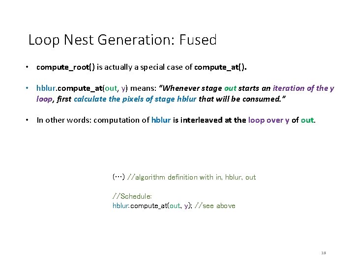
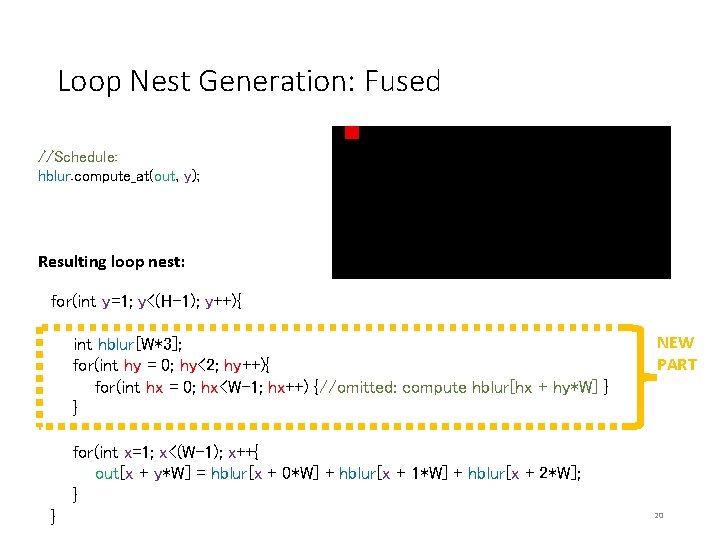
Loop Nest Generation: Fused • compute_root() is actually a special case of compute_at(). • hblur. compute_at(out, y) means: “Whenever stage out starts an iteration of the y loop, first calculate the pixels of stage hblur that will be consumed. ” • In other words: computation of hblur is interleaved at the loop over y of out. (…) //algorithm definition with in, hblur, out //Schedule: hblur. compute_at(out, y); //see above 18

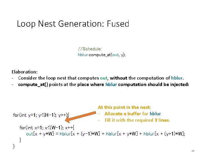
Loop Nest Generation: Fused //Schedule: hblur. compute_at(out, y); Elaboration: - Consider the loop nest that computes out, without the computation of hblur. - compute_at() points at the place where hblur computation should be injected: for(int y=1; y<(H-1); y++){ At this point in the nest: - Allocate a buffer for hblur - Fill it with the required 3 lines. for(int x=1; x<(W-1); x++{ out[x + y*W] = hblur[x + (y-1)*W] + hblur[x + y*W] + hblur[x + (y+1)*W]; } } 19

Loop Nest Generation: Fused //Schedule: hblur. compute_at(out, y); Resulting loop nest: for(int y=1; y<(H-1); y++){ int hblur[W*3]; for(int hy = 0; hy<2; hy++){ for(int hx = 0; hx<W-1; hx++) {//omitted: compute hblur[hx + hy*W] } } NEW PART for(int x=1; x<(W-1); x++{ out[x + y*W] = hblur[x + 0*W] + hblur[x + 1*W] + hblur[x + 2*W]; } } 20

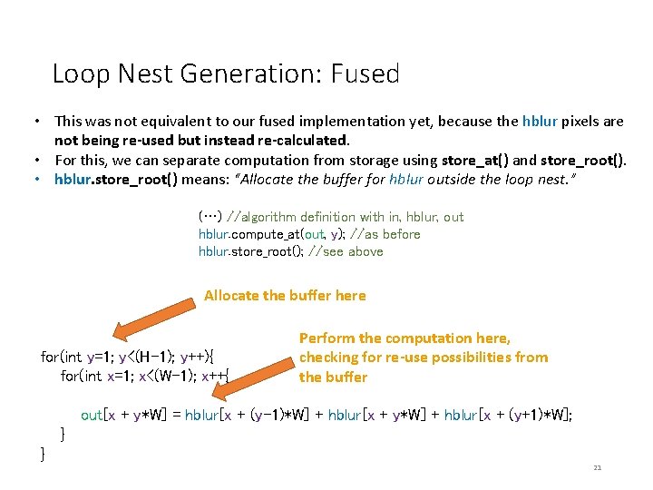
Loop Nest Generation: Fused • This was not equivalent to our fused implementation yet, because the hblur pixels are not being re-used but instead re-calculated. • For this, we can separate computation from storage using store_at() and store_root(). • hblur. store_root() means: “Allocate the buffer for hblur outside the loop nest. ” (…) //algorithm definition with in, hblur, out hblur. compute_at(out, y); //as before hblur. store_root(); //see above Allocate the buffer here for(int y=1; y<(H-1); y++){ for(int x=1; x<(W-1); x++{ Perform the computation here, checking for re-use possibilities from the buffer out[x + y*W] = hblur[x + (y-1)*W] + hblur[x + y*W] + hblur[x + (y+1)*W]; } } 21

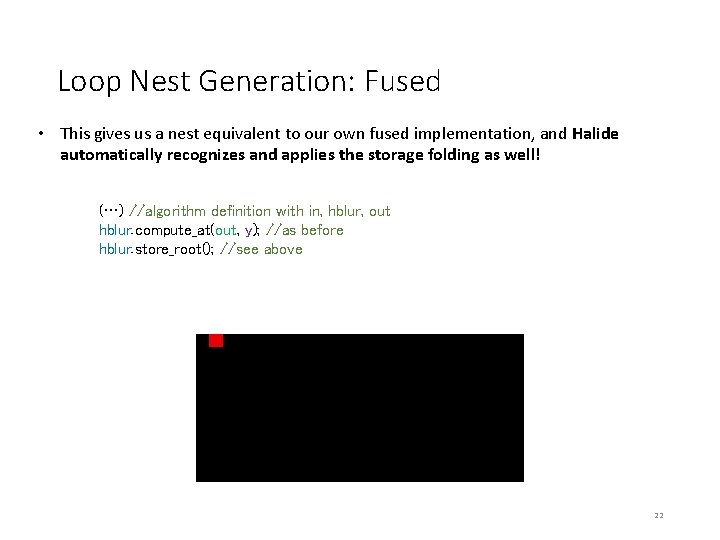
Loop Nest Generation: Fused • This gives us a nest equivalent to our own fused implementation, and Halide automatically recognizes and applies the storage folding as well! (…) //algorithm definition with in, hblur, out hblur. compute_at(out, y); //as before hblur. store_root(); //see above 22

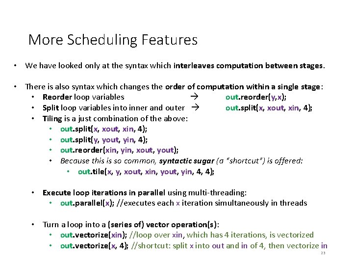
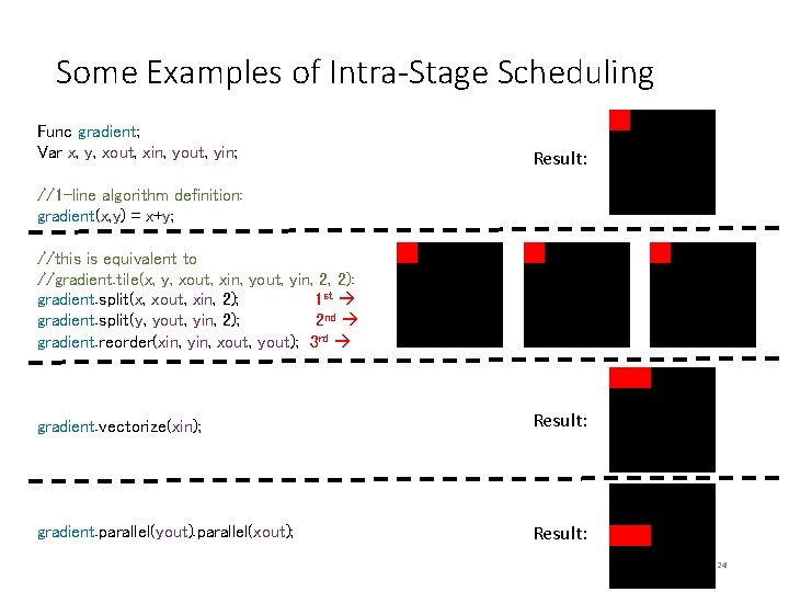
More Scheduling Features • We have looked only at the syntax which interleaves computation between stages. • There is also syntax which changes the order of computation within a single stage: • Reorder loop variables out. reorder(y, x); • Split loop variables into inner and outer out. split(x, xout, xin, 4); • Tiling is a just combination of the above: • out. split(x, xout, xin, 4); • out. split(y, yout, yin, 4); • out. reorder(xin, yin, xout, yout); • Because this is so common, syntactic sugar (a “shortcut”) is offered: • out. tile(x, y, xout, xin, yout, yin, 4, 4); • Execute loop iterations in parallel using multi-threading: • out. parallel(x); //executes each x iteration simultaneously in threads • Turn a loop into a (series of) vector operation(s): • out. vectorize(xin); //loop over xin, which has 4 iterations, is vectorized • out. vectorize(x, 4); //shortcut: split x into out and in of 4, then vectorize in 23

Some Examples of Intra-Stage Scheduling Func gradient; Var x, y, xout, xin, yout, yin; Result: //1 -line algorithm definition: gradient(x, y) = x+y; //this is equivalent to //gradient. tile(x, y, xout, xin, yout, yin, 2, 2): gradient. split(x, xout, xin, 2); 1 st gradient. split(y, yout, yin, 2); 2 nd gradient. reorder(xin, yin, xout, yout); 3 rd gradient. vectorize(xin); Result: gradient. parallel(yout). parallel(xout); Result: 24

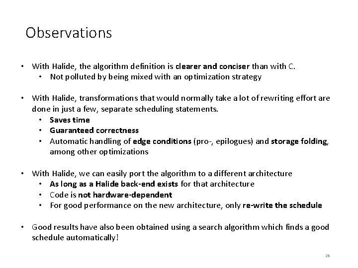
Observations • With Halide, the algorithm definition is clearer and conciser than with C. • Not polluted by being mixed with an optimization strategy • With Halide, transformations that would normally take a lot of rewriting effort are done in just a few, separate scheduling statements. • Saves time • Guaranteed correctness • Automatic handling of edge conditions (pro-, epilogues) and storage folding, among other optimizations • With Halide, we can easily port the algorithm to a different architecture • As long as a Halide back-end exists for that architecture • Code is not hardware-dependent • For good performance on the new architecture, only re-write the schedule • Good results have also been obtained using a search algorithm which finds a good schedule automatically! 25

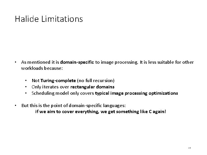
Halide Limitations • As mentioned it is domain-specific to image processing. It is less suitable for other workloads because: • Not Turing-complete (no full recursion) • Only iterates over rectangular domains • Scheduling model only covers typical image processing optimizations • But this is the point of domain-specific languages: if we aim to cover everything, we get something like C again! 26

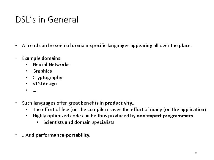
DSL’s in General • A trend can be seen of domain-specific languages appearing all over the place. • Example domains: • Neural Networks • Graphics • Cryptography • VLSI design • … • Such languages offer great benefits in productivity… • The effort of few (on the compiler) saves the effort of many (on the application) • Highly optimized code can be thus produced by non-expert programmers • Scientists and domain specialists • …And performance-portability. 27

Halide’s Status • An open-source project. • Because of that, there is ongoing work in many directions: • New architectures (DSPs, supercomputers…) • Extensions to suit (sub-)domains • Auxiliary efforts: • Automatic tuning of Halide schedules • Automatic generating of Halide schedules • Automatic de-compilation of x 86 binaries into Halide for easy porting • Support from Google in the industry 28

Preview of next time (March 31 st) • How does the Halide compiler leverage LLVM and C++? • What does Halide’s IR look like? How to operate on it? • What do Halide’s code generator back-ends look like? • How does Halide move from functional-style input to imperative (assembly-style) output? • …And more (TBD) 29

? 30