Introduction to Graphing in SAS Greg Grandits Division

Introduction to Graphing in SAS Greg Grandits, Division of Biostatistics March 6, 2017 www. biostat. umn. edu/~greg-g/ph 6344. html

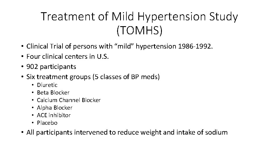
Treatment of Mild Hypertension Study (TOMHS) • • Clinical Trial of persons with “mild” hypertension 1986 -1992. Four clinical centers in U. S. 902 participants Six treatment groups (5 classes of BP meds) • • • Diuretic Beta Blocker Calcium Channel Blocker Alpha Blocker ACE inhibitor Placebo • All participants intervened to reduce weight and intake of sodium

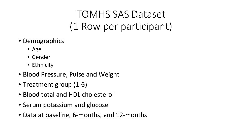
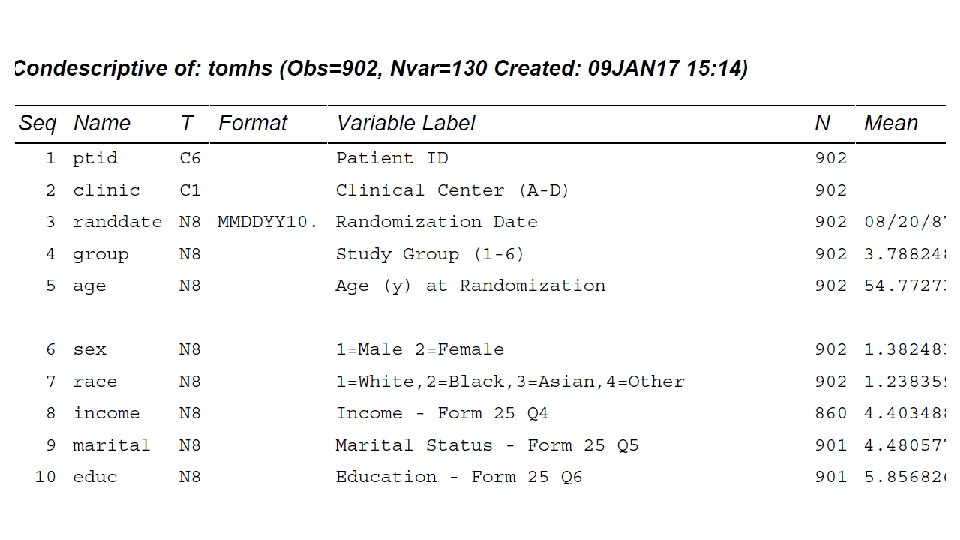
TOMHS SAS Dataset (1 Row per participant) • Demographics • Age • Gender • Ethnicity • Blood Pressure, Pulse and Weight • Treatment group (1 -6) • Blood total and HDL cholesterol • Serum potassium and glucose • Data at baseline, 6 -months, and 12 -months

Graphing With SAS • PROC SGPLOT • • • Histograms Box plots Barcharts Scatter plots (regression line) Series plots • PROC SGPANEL • Paneled plots • Example: Boxplots of Change in BP by Group, Paneled by visit

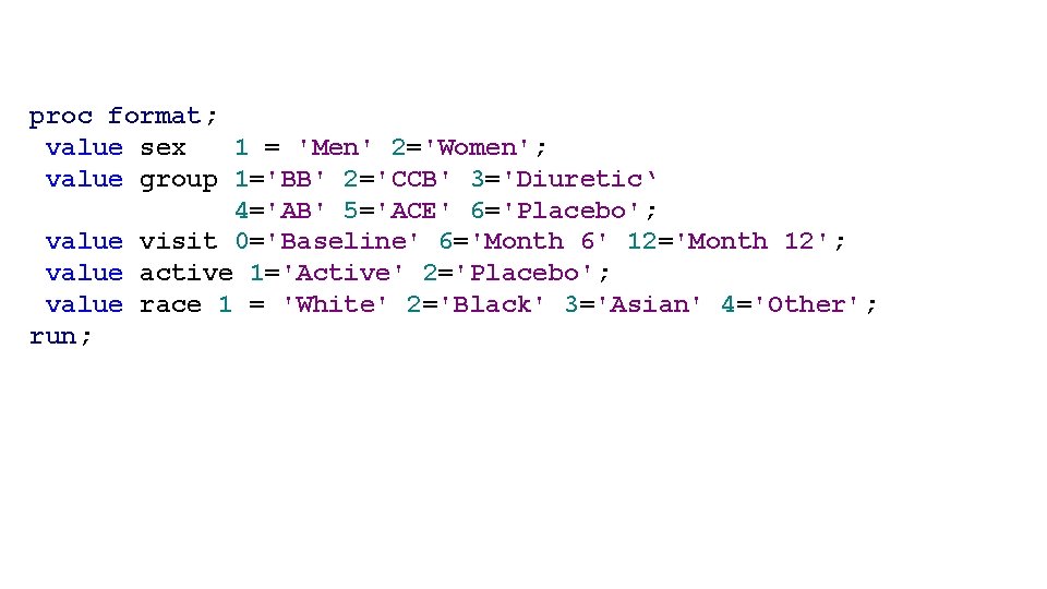
proc format; value sex 1 = 'Men' 2='Women'; value group 1='BB' 2='CCB' 3='Diuretic‘ 4='AB' 5='ACE' 6='Placebo'; value visit 0='Baseline' 6='Month 6' 12='Month 12'; value active 1='Active' 2='Placebo'; value race 1 = 'White' 2='Black' 3='Asian' 4='Other'; run;

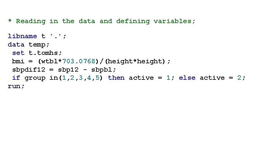
* Reading in the data and defining variables; libname t '. '; data temp; set t. tomhs; bmi = (wtbl*703. 0768)/(height*height); sbpdif 12 = sbp 12 - sbpbl; if group in(1, 2, 3, 4, 5) then active = 1; else active = 2; run;

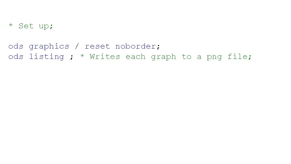
* Set up; ods graphics / reset noborder; ods listing ; * Writes each graph to a png file;

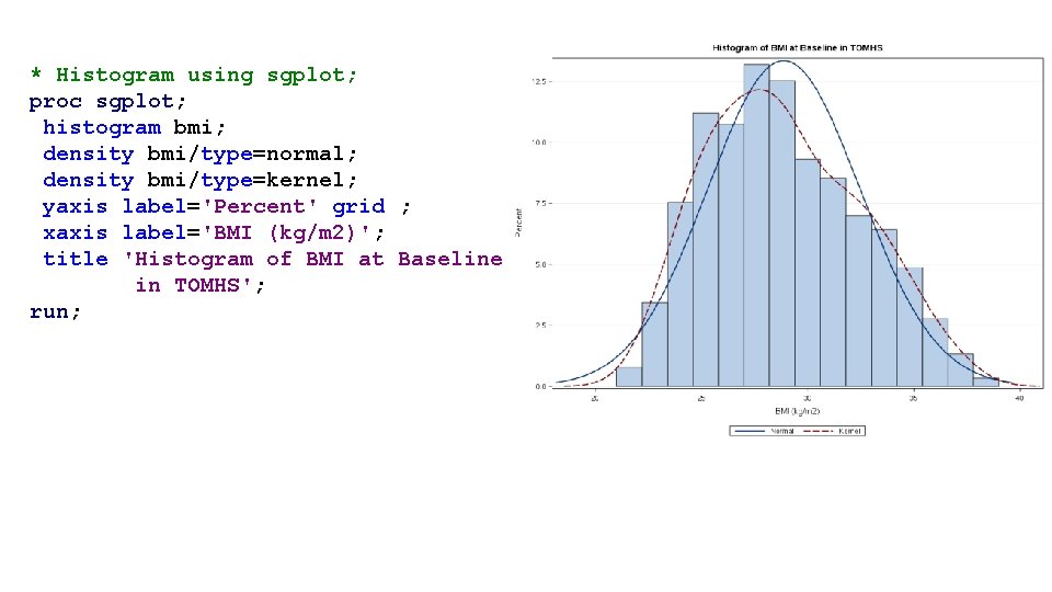
* Histogram using sgplot; proc sgplot; histogram bmi; density bmi/type=normal; density bmi/type=kernel; yaxis label='Percent' grid ; xaxis label='BMI (kg/m 2)'; title 'Histogram of BMI at Baseline in TOMHS'; run;

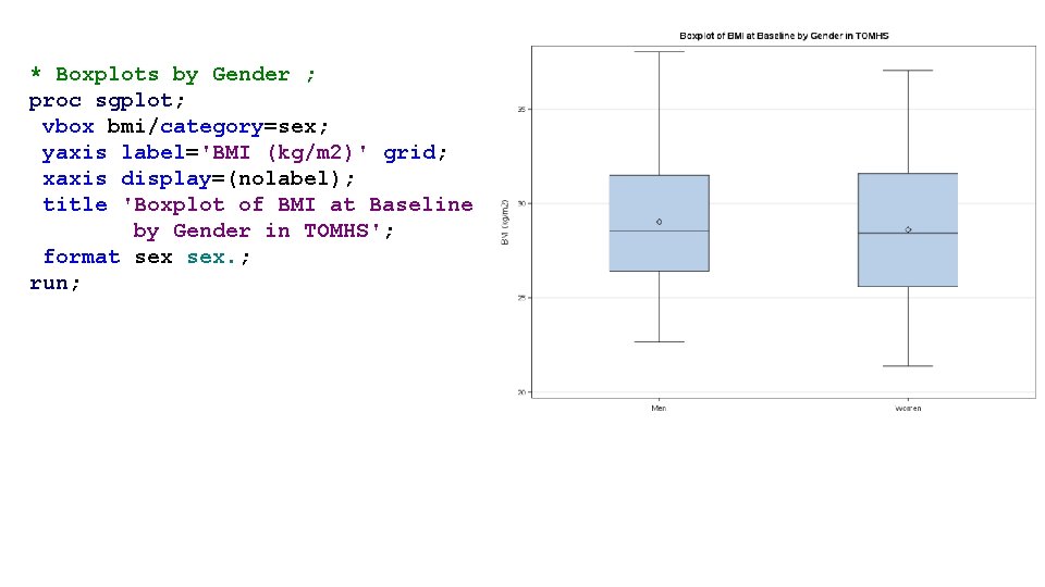
* Boxplots by Gender ; proc sgplot; vbox bmi/category=sex; yaxis label='BMI (kg/m 2)' grid; xaxis display=(nolabel); title 'Boxplot of BMI at Baseline by Gender in TOMHS'; format sex. ; run;

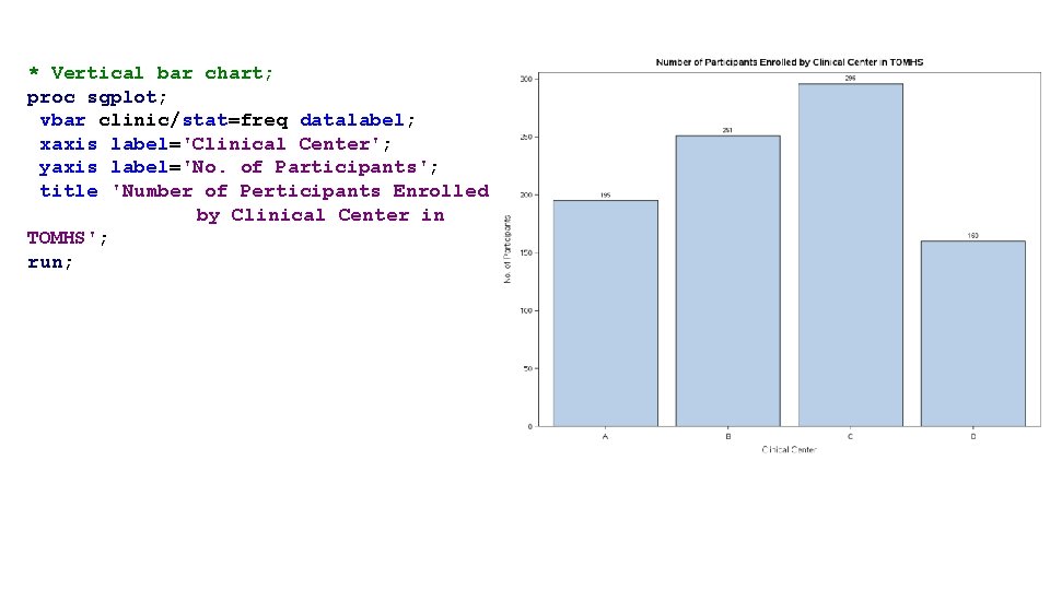
* Vertical bar chart; proc sgplot; vbar clinic/stat=freq datalabel; xaxis label='Clinical Center'; yaxis label='No. of Participants'; title 'Number of Perticipants Enrolled by Clinical Center in TOMHS'; run;

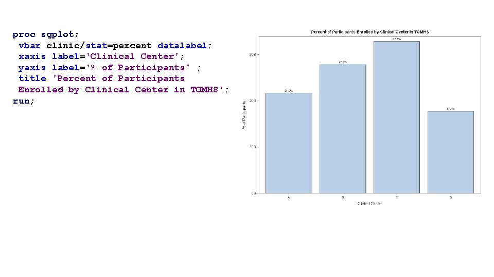
proc sgplot; vbar clinic/stat=percent datalabel; xaxis label='Clinical Center'; yaxis label='% of Participants' ; title 'Percent of Participants Enrolled by Clinical Center in TOMHS'; run;

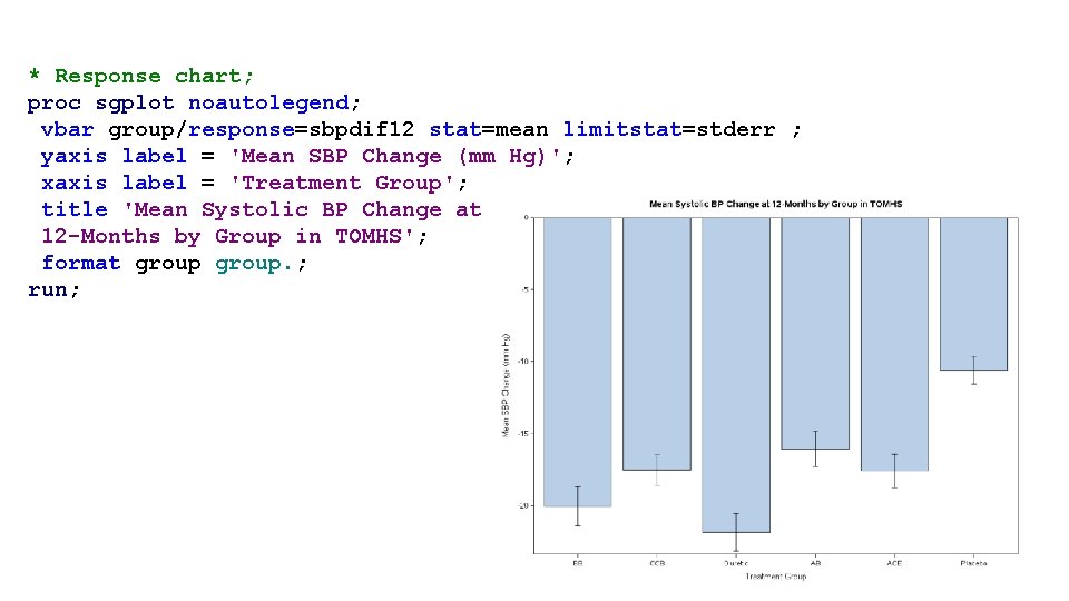
* Response chart; proc sgplot noautolegend; vbar group/response=sbpdif 12 stat=mean limitstat=stderr ; yaxis label = 'Mean SBP Change (mm Hg)'; xaxis label = 'Treatment Group'; title 'Mean Systolic BP Change at 12 -Months by Group in TOMHS'; format group. ; run;

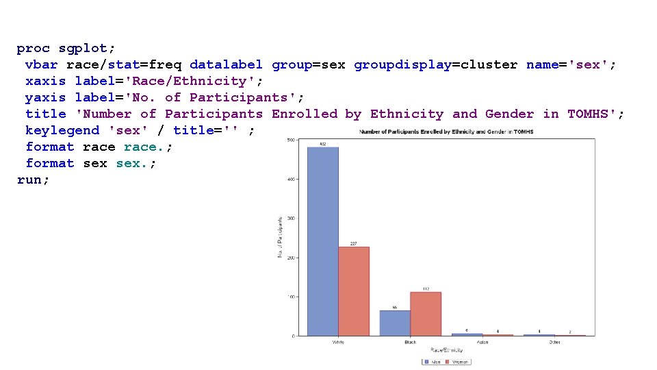
proc sgplot; vbar race/stat=freq datalabel group=sex groupdisplay=cluster name='sex'; xaxis label='Race/Ethnicity'; yaxis label='No. of Participants'; title 'Number of Participants Enrolled by Ethnicity and Gender in TOMHS'; keylegend 'sex' / title='' ; format race. ; format sex. ; run;

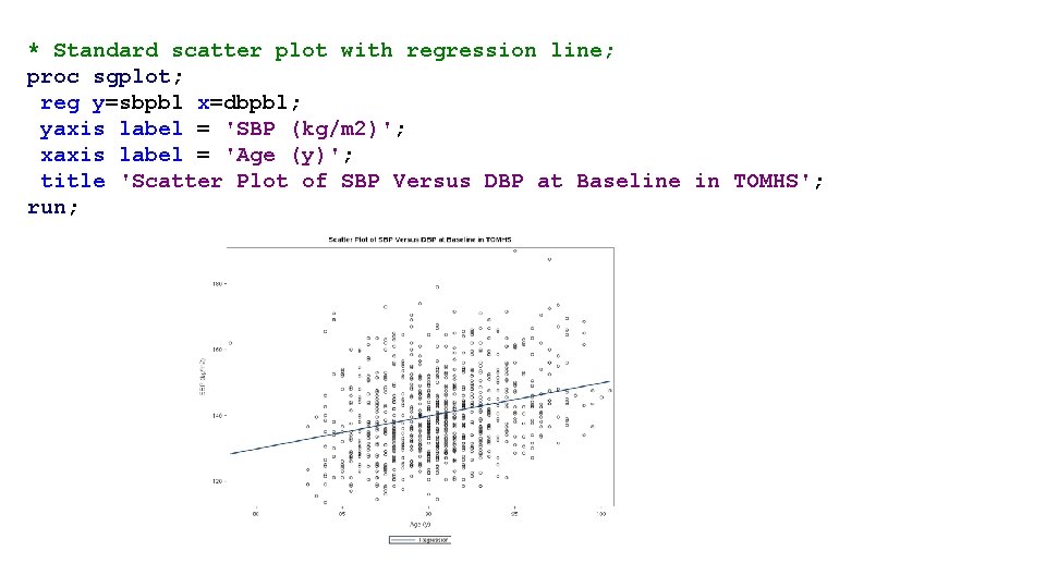
* Standard scatter plot with regression line; proc sgplot; reg y=sbpbl x=dbpbl; yaxis label = 'SBP (kg/m 2)'; xaxis label = 'Age (y)'; title 'Scatter Plot of SBP Versus DBP at Baseline in TOMHS'; run;

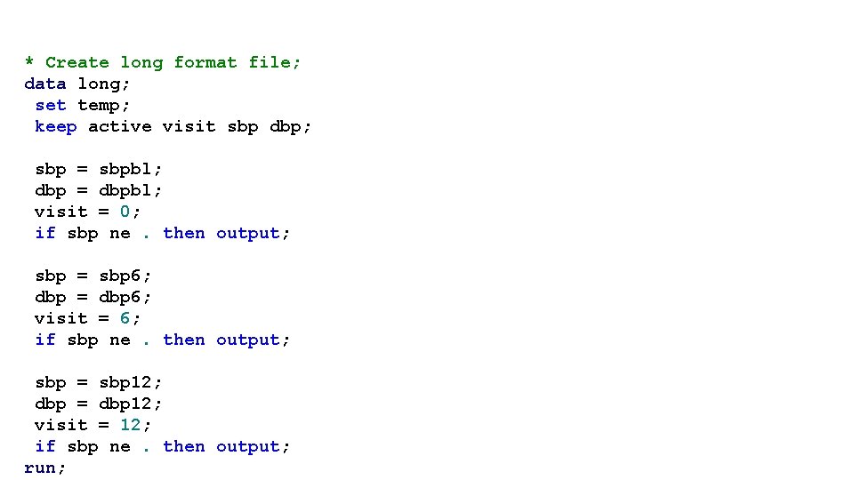
* Create long format file; data long; set temp; keep active visit sbp dbp; sbp = sbpbl; dbp = dbpbl; visit = 0; if sbp ne. then output; sbp = sbp 6; dbp = dbp 6; visit = 6; if sbp ne. then output; sbp = sbp 12; dbp = dbp 12; visit = 12; if sbp ne. then output; run;

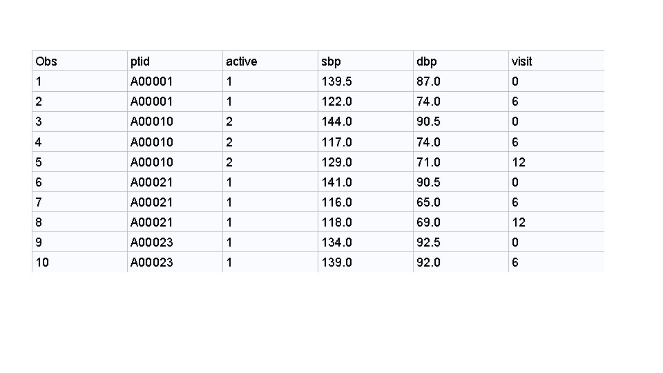
Obs ptid active sbp dbp visit 1 A 00001 1 139. 5 87. 0 0 2 A 00001 1 122. 0 74. 0 6 3 A 00010 2 144. 0 90. 5 0 4 A 00010 2 117. 0 74. 0 6 5 A 00010 2 129. 0 71. 0 12 6 A 00021 1 141. 0 90. 5 0 7 A 00021 1 116. 0 65. 0 6 8 A 00021 1 118. 0 69. 0 12 9 A 00023 1 134. 0 92. 5 0 10 A 00023 1 139. 0 92. 0 6

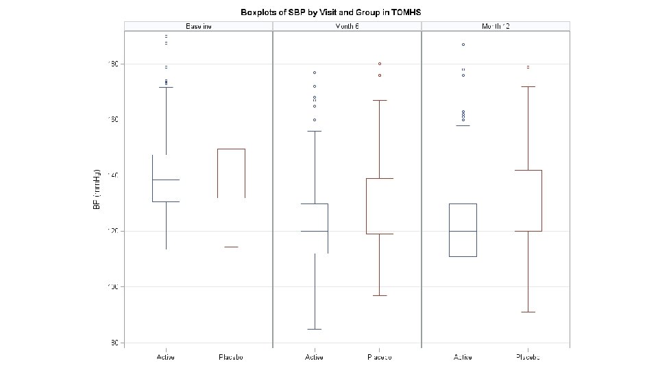
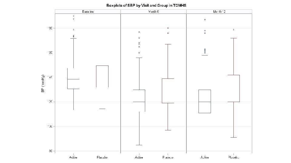
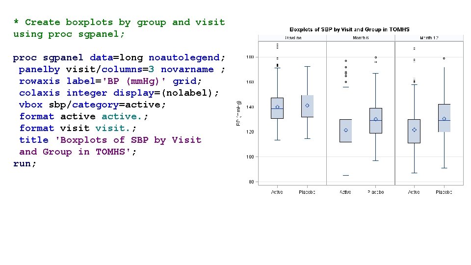
* Create boxplots by group and visit using proc sgpanel; proc sgpanel data=long noautolegend; panelby visit/columns=3 novarname ; rowaxis label='BP (mm. Hg)' grid; colaxis integer display=(nolabel); vbox sbp/category=active; format active. ; format visit. ; title 'Boxplots of SBP by Visit and Group in TOMHS'; run;

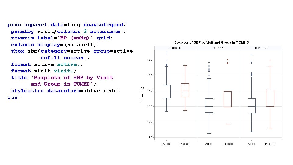
proc sgpanel data=long noautolegend; panelby visit/columns=3 novarname ; rowaxis label='BP (mm. Hg)' grid; colaxis display=(nolabel); vbox sbp/category=active group=active nofill nomean ; format active. ; format visit. ; title 'Boxplots of SBP by Visit and Group in TOMHS'; styleattrs datacolors=(blue red); run;

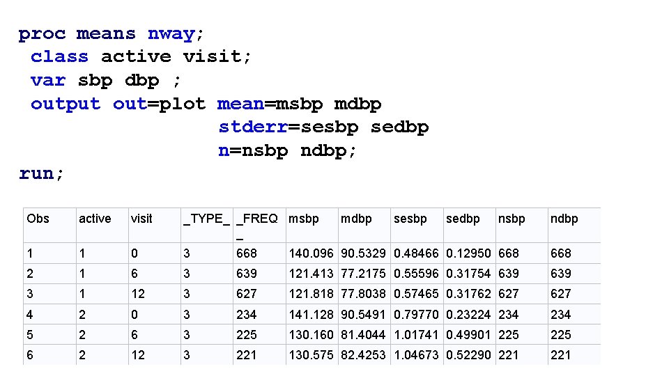
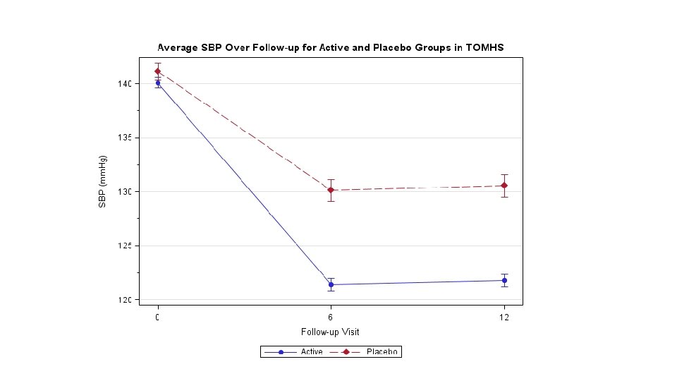
proc means nway; class active visit; var sbp dbp ; output out=plot mean=msbp mdbp stderr=sesbp sedbp n=nsbp ndbp; run; Obs active visit _TYPE_ _FREQ msbp _ mdbp sesbp sedbp nsbp ndbp 1 1 0 3 668 140. 096 90. 5329 0. 48466 0. 12950 668 2 1 6 3 639 121. 413 77. 2175 0. 55596 0. 31754 639 3 1 12 3 627 121. 818 77. 8038 0. 57465 0. 31762 627 4 2 0 3 234 141. 128 90. 5491 0. 79770 0. 23224 234 5 2 6 3 225 130. 160 81. 4044 1. 01741 0. 49901 225 6 2 12 3 221 130. 575 82. 4253 1. 04673 0. 52290 221

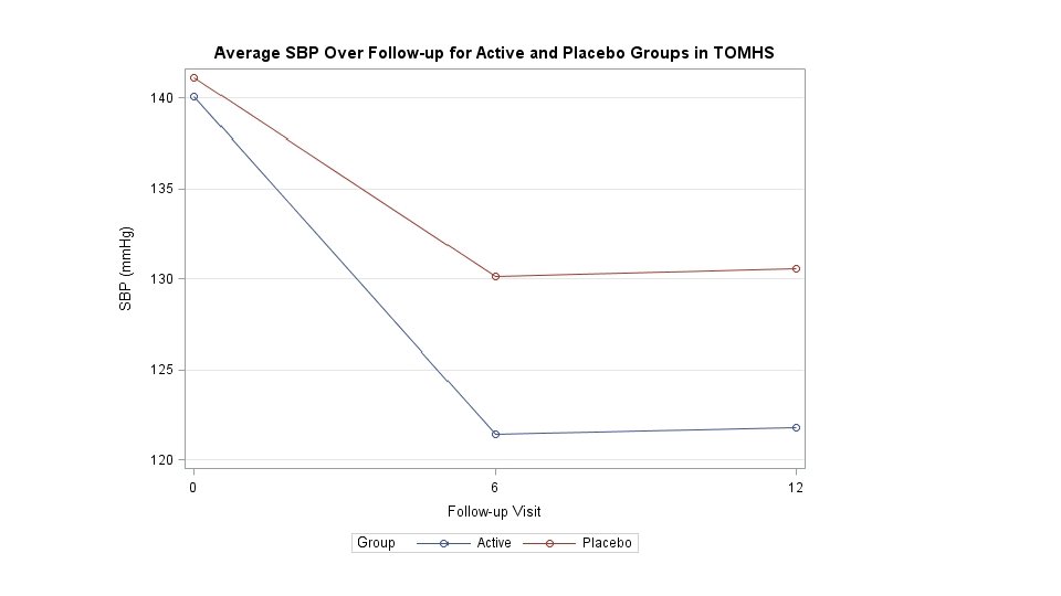
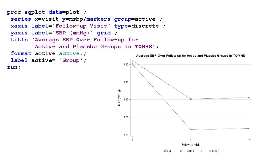
proc sgplot data=plot ; series x=visit y=msbp/markers group=active ; xaxis label='Follow-up Visit' type=discrete ; yaxis label='SBP (mm. Hg)' grid ; title 'Average SBP Over Follow-up for Active and Placebo Groups in TOMHS'; format active. ; label active= 'Group'; run;

data plot; set plot (drop=_freq_ _type_); uppsbp = msbp + sesbp; lowsbp = msbp - sesbp; uppdbp = mdbp + sedbp; lowdbp = mdbp - sedbp; run;

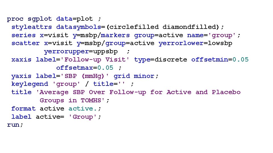
proc sgplot data=plot ; styleattrs datasymbols=(circlefilled diamondfilled); series x=visit y=msbp/markers group=active name='group'; scatter x=visit y=msbp/group=active yerrorlower=lowsbp yerrorupper=uppsbp ; xaxis label='Follow-up Visit' type=discrete offsetmin=0. 05 offsetmax=0. 05 ; yaxis label='SBP (mm. Hg)' grid minor; keylegend 'group' / title='' ; title 'Average SBP Over Follow-up for Active and Placebo Groups in TOMHS'; format active. ; label active= 'Group'; run;