Introduction to GMT Part 2 Matt Herman Last

Introduction to GMT (Part 2) Matt Herman Last updated: 27 November 2020

Tutorial Objectives • Learn the following new GMT commands • grdimage • makecpt • psscale • grdcontour • surface Note: This tutorial assumes knowledge from Part 1. If you are a new user, you may want to go back and complete Part 1 first!

Outline of Tutorial Activities • grdimage: topography • grdimage + makecpt + psscale: ocean floor age • grdcontour: subduction interface depth • surface: interpolate GPS data

Raster Files • In the first installment, we plotted point data, like coastlines and earthquakes • Some datasets are collected over large areas, so it is better to treat them as swath observations rather than point data • GMT uses a standard format for these datasets called Net. CDF • These files often (but not always!) have the extension *. grd

Introduction to grdimage gmt grdimage ETOPO 5. grd -JM 5 i -R-130/-60/20/55 > topo_0. ps gmt grdimage The command grdimage produces an image on your map from a Net. CDF file. ETOPO 5. grd The first argument must be the name of a Net. CDF file. In this case, we are plotting topography, so the file is ETOPO 5, a global topography/bathymetry dataset at 5 arcminute (1/12 degree) resolution. You can download the ETOPO 5 file from my Tutorials page or directly from NOAA (https: //www. ngdc. noaa. gov/mgg/global/etop o 5. HTML) Data Announcement 88 -MGG-02, Digital relief of the Surface of the Earth. NOAA, National Geophysical Data Center, Boulder, Colorado, 1988.

Introduction to grdimage gmt grdimage ETOPO 5. grd -JM 5 i -R-130/-60/20/55 > topo_0. ps Although you may be able to tell from this figure that the map contains the topography of the United States, it is difficult to see details. By default, grdimage will use the rainbow color palette (objectively terrible) and stretch it to the limits of the dataset. Next, we will apply a different pre-installed color palette that makes the topography look better. Data Announcement 88 -MGG-02, Digital relief of the Surface of the Earth. NOAA, National Geophysical Data Center, Boulder, Colorado, 1988.

Introduction to grdimage gmt grdimage ETOPO 5. grd -JM 5 i -R-130/-60/20/55 -Ctopo > topo_1. ps -Ctopo The option -C tells grdimage to use a different color palette. GMT has several builtin options, including this topography palette designed by David Sandwell. This approach can be great for quick looks at datasets, but for nicer productions you will typically want to use a color palette that fits the specific needs of your figure. Add the -C option to the command

Using grdimage, we will make this figure with a custom topography color palette.

1. Put this text into a file named “topo 2. cpt”. This is a color palette I -27000 0/28/74 -6000 0/28/74 borrowed from Dr. -6000 0/68/129 -5000 0/68/129 -5000 0/102/166 -4000 0/102/166 Charles Ammon at -4000 80/143/193 -3000 130/181/217 -2000 130/181/217 Penn State. -2000 178/207/231 -1000 153/204/255 -1000 208/236/243 -500 255/255/255 0 100/150/100 30 125/175/125 60 150/200/150 122 175/225/175 183 200/255/200 244 212/255/212 305 255/255/225 457 255/225/175 610 255/225/125 702 255/175/75 914 255/175/75 914 200/150/50 1219 175/125/50 1450 150/100/50 1700 150/125/100 1981 125/125/125 2134 150/150/150 2438 175/175/175 2743 200/200/200 3048 233/233 3250 233/233

1. Put this text into a file named “topo 2. cpt”. This is a color palette I -27000 0/28/74 -6000 0/28/74 borrowed from Dr. -6000 0/68/129 -5000 0/68/129 -5000 0/102/166 -4000 0/102/166 Charles Ammon at -4000 80/143/193 -3000 130/181/217 -2000 130/181/217 Penn State. -2000 178/207/231 -1000 153/204/255 Each line in a GMT color palette file is a color slice and must contain: starting value starting color (red/green/blue) ending value ending color (red/green/blue) -1000 208/236/243 -500 255/255/255 0 100/150/100 30 125/175/125 60 150/200/150 122 175/225/175 183 200/255/200 244 212/255/212 305 255/255/225 457 255/225/175 610 255/225/125 702 255/175/75 914 255/175/75 914 200/150/50 1219 175/125/50 1450 150/100/50 1700 150/125/100 1981 125/125/125 2134 150/150/150 2438 175/175/175 2743 200/200/200 3048 233/233 3250 233/233 The values must be continuous from line to line. Starting Ending Elevation Color

1. Put this text into a file named “topo 2. cpt”. This is a color palette I -27000 0/28/74 -6000 0/28/74 borrowed from Dr. -6000 0/68/129 -5000 0/68/129 -5000 0/102/166 -4000 0/102/166 Charles Ammon at -4000 80/143/193 -3000 130/181/217 -2000 130/181/217 Penn State. -2000 178/207/231 -1000 153/204/255 2. Make a script with the grdimage command add a coastline and basemap (using pscoast and psbasemap from the previous tutorial). PSFILE=“topo_2. ps” PROJ=“-JM 8 i” LIMS=“-R-130/-60/20/55” -1000 208/236/243 -500 255/255/255 0 100/150/100 30 125/175/125 60 150/200/150 122 175/225/175 183 200/255/200 244 212/255/212 305 255/255/225 457 255/225/175 610 255/225/125 702 255/175/75 914 255/175/75 914 200/150/50 1219 175/125/50 1450 150/100/50 1700 150/125/100 1981 125/125/125 2134 150/150/150 2438 175/175/175 2743 200/200/200 3048 233/233 3250 233/233 gmt grdimage ETOPO 5. grd $PROJ $LIMS -Ctopo 2. cpt -K > $PSFILE gmt pscoast $PROJ $LIMS -Dl -W 1 p -N 1/1 p -K -O >> $PSFILE gmt psbasemap $PROJ $LIMS -Bxa 10 -Bya 10 -BWe. Sn -O >> $PSFILE

1. Put this text into a file named “topo 2. cpt”. This is a color palette I -27000 0/28/74 -6000 0/28/74 borrowed from Dr. -6000 0/68/129 -5000 0/68/129 -5000 0/102/166 -4000 0/102/166 Charles Ammon at -4000 80/143/193 -3000 130/181/217 -2000 130/181/217 Penn State. -2000 178/207/231 -1000 153/204/255 2. Make a script with the grdimage command add a coastline and basemap (using pscoast and psbasemap from the previous tutorial). PSFILE=“topo_2. ps” PROJ=“-JM 8 i” LIMS=“-R-130/-60/20/55” 3. Use the new color palette for the topography -1000 208/236/243 -500 255/255/255 0 100/150/100 30 125/175/125 60 150/200/150 122 175/225/175 183 200/255/200 244 212/255/212 305 255/255/225 457 255/225/175 610 255/225/125 702 255/175/75 914 255/175/75 914 200/150/50 1219 175/125/50 1450 150/100/50 1700 150/125/100 1981 125/125/125 2134 150/150/150 2438 175/175/175 2743 200/200/200 3048 233/233 3250 233/233 gmt grdimage ETOPO 5. grd $PROJ $LIMS -Ctopo 2. cpt -K > $PSFILE gmt pscoast $PROJ $LIMS -Dl -W 1 p -N 1/1 p -K -O >> $PSFILE gmt psbasemap $PROJ $LIMS -Bxa 10 -Bya 10 -BWe. Sn -O >> $PSFILE

Excellent! You can now make a nice topography/bathymetry map.

Next we will practice using grdimage on a different dataset (ocean floor age), while we also learn to use the commands makecpt and psscale.

Introduction to makecpt This Net. CDF file ends in. nc instead of. grd like the topography dataset gmt grdimage ocean_age. nc -JM 6 i -R-40/10/-40/0 > age_1. ps First, plot the ocean floor age dataset for the South Atlantic Ocean using the default colors. You can find the data clipped to the region shown in the map at this link, or the full data from the source (NOAA again): https: //www. ngdc. noaa. gov/mgg/ocean_age/ data/2008/grids/age As you might expect, this is not a useful figure because if we do not already know, the figure does not tell us anything about what is on it! Muller, R. D. , M. Sdrolias, C. Gaina, and W. R. Roest (2008), Age, spreading rates, and spreading asymmetry of the world’s ocean crust, Geochem. Geophys. Geosyst. , 9, Q 04006

Introduction to makecpt Now we need to define the new color palette in the grdimage options gmt makecpt -T 0/120/10 > age. cpt gmt grdimage ocean_age. nc -JM 6 i -R-40/10/-40/0 -Cage. cpt > age_2. ps gmt makecpt If we want more control over our color schemes but do not want to create a palette from scratch, we can use makecpt. It takes an existing color palette (either a GMT built-in or a file) and stretches it to fit a new range. -T 0/120/10 The range and increment of the new, output color palette is defined by the -T option. It is followed by the minimum value, maximum value, and increment. This age of the ocean in the South Atlantic spans 0 to ~120 million years, so this is an appropriate range for the color palette.

Introduction to makecpt gmt makecpt -T 0/120/10 > age. cpt gmt grdimage ocean_age. nc -JM 6 i -R-40/10/-40/0 -Cage. cpt > age_2. ps As I said earlier, the rainbow color palette is crappy. Look at the green areas. Are those wider because spreading increased in velocity during that time period? Let us use a better color map to tell for sure.

Introduction to makecpt gmt makecpt -Cinferno -T 0/120/10 > age. cpt gmt grdimage ocean_age. nc -JM 6 i -R-40/10/-40/0 -Cage. cpt > age_3. ps -Cinferno GMT has many built-in color palettes available, including 4 perceptually linear (good!) schemes called Viridis, Inferno, Magma, and Plasma. You can see the names of all of the built-in color maps by running “makecpt” with no options. Using this perceptually linear color map, we can see that the spreading rate has not changed as much as the wide green regions from the previous figure might suggest.

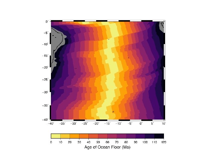
Introduction to makecpt gmt makecpt -Cinferno -T 0/120/10 -I > age. cpt gmt grdimage ocean_age. nc -JM 6 i -R-40/10/-40/0 -Cage. cpt > age_4. ps In this case, it makes more sense to have younger, warmer ocean near ridges be a brighter color than the colder, older ocean near Africa and South America. -I To invert the color scheme, use the -I option.

Introduction to psscale New command to make a scale bar. gmt grdimage ocean_age. nc -JM 6 i -R-40/10/-40/0 -Cage. cpt -K > age_5. ps gmt psscale -D 0/-3+w 10/0. 5+h -Cage. cpt -Ba 10+l”Age” -O >> age_5. ps gmt psscale A color palette is most useful when the viewer knows what the color represent. It is common to provide this information in a scale bar of some kind. Plot a scale bar on the figure with psscale. -D 0/-3+w 10/0. 5+h Define the location and dimensions of the scale bar with -D. The position of the bottom left of the scale bar (in cm) relative to the bottom left of your map region is the first two coordinates (0/-3) and the size of the scale bar is the two values after +w (10/0. 5). By default, the bar is vertical. To turn it horizontal, we add +h.

Introduction to psscale gmt grdimage ocean_age. nc -JM 6 i -R-40/10/-40/0 -Cage. cpt -K > age_5. ps gmt psscale -D 0/-3+w 10/0. 5+h -Cage. cpt -Ba 10+l”Age” -O >> age_5. ps -Cage. cpt The scale bar will use the color palette defined with the -C option, just like grdimage. -Ba 10+l”Age” The syntax for annotating the scale bar is very similar to that of psbasemap, and uses the same -B option. Here, we are annotating the scale bar every 10 increments (million years) and labeling it with the string “Age. ”

PSFILE=“ocean_age. ps” PROJ=“-JM 6 i” LIMS=“-R-40/10/-40/0” Plotting variables Color palette range # Age in millions of years AGE_MIN=“ 0” Make color palette AGE_MAX=“ 120” gmt makecpt -Cinferno -T$AGE_MIN/$AGE_MAX/10 -D -I > age. cpt Plot ocean age gmt grdimage ocean_age. nc $PROJ $LIMS -Cage. cpt -Y 2 i -K > $PSFILE Plot coastlines gmt pscoast $PROJ $LIMS -Di -W 1 p -K -O >> $PSFILE gmt psbasemap $PROJ $LIMS -Bxa 5 -Bya 5 -BWe. Sn -K -O >> $PSFILE Plot map frame gmt psscale -D 0 i/-1 i+w 6 i/0. 25 i+h -Cage. cpt -Bg 10 a 10+l”Age of Ocean Floor (Ma)” -O >> $PSFILE Plot scale bar A basic shell script for plotting ocean age

Introduction to grdcontour gmt grdimage sam_slab. grd -JM 5 i -R 280/300/-35/-10 > slab_0. ps Next, we will plot the depth of the subduction plate interface beneath the western coast of South America. Start by using grdimage with the default coloring option. Again, this gives us very little actual information. . . The data come from Slab 1. 0 (Hayes et al. , 2012). You can download the clipped grid file from my Tutorials page or the full dataset (along with other subduction zones) directly from the U. S. Geological Survey (https: //earthquake. usgs. gov/data/slab) Hayes, G. P. , Wald, D. J. , Johnson, R. L. (2012). Slab 1. 0: A three-dimensional model of global subduction zone geometries. Journal of Geophysical Research, 117, B 01302. http: //doi. org/10. 1029/2011 JB 008524

Introduction to grdcontour gmt grdcontour sam_slab. grd -JM 5 i -R 280/300/-35/-10 -C 25 -W 1 p > slab_1. ps gmt grdcontour Another common way to show 3 D raster data is with contour lines. GMT can do this for Net. CDF files with the command grdcontour. -C 25 The contour interval is specified using the -C option. The value you choose depends on the range of the dataset you want to plot. Here, the interface extends from 0 km to over 400 km, so I chose to use an interval of 25 m, which shows the shallow dip near the trench and the much steeper angle at depth. Hayes, G. P. , Wald, D. J. , Johnson, R. L. (2012). Slab 1. 0: A three-dimensional model of global subduction zone geometries. Journal of Geophysical Research, 117, B 01302. http: //doi. org/10. 1029/2011 JB 008524

Introduction to grdcontour gmt grdcontour sam_slab. grd -JM 5 i -R 280/300/-35/-10 -C 25 -W 1 p -A 100 > slab_2. ps -A 100 It is important to label the contour lines. The A option allows you to define a constant annotation interval, here 100 m. Hayes, G. P. , Wald, D. J. , Johnson, R. L. (2012). Slab 1. 0: A three-dimensional model of global subduction zone geometries. Journal of Geophysical Research, 117, B 01302. http: //doi. org/10. 1029/2011 JB 008524

Introduction to grdcontour gmt grdcontour sam_slab. grd -JM 5 i -R 280/300/-35/-10 -C 25 -W 1 p -A 100 -Gd 4 c > slab_3. ps -Gd 4 c Maybe you found it difficult to trace the labeled contours in the previous figure, like I did. To adjust the labeling, you can use the -G option. There are many variations (see the grdcontour man page for details), but by using d 4 c I have told the program to plot a label every 4 cm, making it easier to trace the contours along the entire length. Hayes, G. P. , Wald, D. J. , Johnson, R. L. (2012). Slab 1. 0: A three-dimensional model of global subduction zone geometries. Journal of Geophysical Research, 117, B 01302. http: //doi. org/10. 1029/2011 JB 008524

Introduction to grdcontour gmt grdcontour sam_slab. grd -JM 5 i -R 280/300/-35/-10 -C 25 -W 0. 5 p, grey 50 -K > slab_4. ps gmt grdcontour sam_slab. grd -J -R -C 100 -W 2 p -A 100 -Gd 4 c -O >> slab_4. ps I find that using grdcontour multiple times with different options gives me the most control over the appearance of the map. Here, I used grdcontour twice: once to draw the 25 m contours in a light grey pen and another time to boldly draw the 100 m labeled contours. Hayes, G. P. , Wald, D. J. , Johnson, R. L. (2012). Slab 1. 0: A three-dimensional model of global subduction zone geometries. Journal of Geophysical Research, 117, B 01302. http: //doi. org/10. 1029/2011 JB 008524

Combining contour lines with colors allow you to put multiple datasets on the same figure. Here, I have plotted topography and bathymetry with grdimage and the depth of the subduction interface with grdcontour. The script for producing this map is on the following slide.

A new color palette for topography with more muted colors. Borrowed from Dr. Gavin Hayes at the USGS. -7500 81/101/153 -6750 88/112/157 -5000 96/129/163 -3750 118/157/179 -2500 131/173/189 -100 137/181/193 0 255/255 0 105/155/105 50 100/150/100 3250 255/235/193 B 60/70/135 F 255/235/193 PSFILE=“south_america. ps” PROJ=“-JM 5 i” LIMS=“-R 280/300/-35/-10” gmt grdimage ETOPO 5. grd $PROJ $LIMS -Ctopo 2. cpt -K > $PSFILE gmt grdcontour sam_slab. grd $PROJ $LIMS -C 25 -W 0. 5 p, grey 50 -K -O >> $PSFILE gmt grdcontour sam_slab. grd $PROJ $LIMS -C 100 -A 100 -Gd 4 c -W 1 p -K -O >> $PSFILE gmt pscoast $PROJ $LIMS -W 0. 5 p, 55/55/55 -Dh -K -O >> $PSFILE gmt psbasemap $PROJ $LIMS -Bxa 2 -Bya 2 -BWe. Sn -O >> $PSFILE

In the last activity for this tutorial, we will make this colored map of displacements observed during the 2011 moment magnitude Mw 9. 1 Tohoku earthquake offshore of Japan. You can use this color palette or make your own! (Name it “disp. cpt”) 0. 0 255. 000/255. 000/254. 981 0. 5 215. 708/233. 215/251. 691 1. 0 190. 815/207. 612/248. 689 1. 5 184. 130/177. 949/239. 358 2. 0 192. 174/143. 781/218. 428 2. 5 204. 929/104. 100/183. 141 3. 0 211. 927/54. 746/134. 139 3. 5 195. 963/0. 397/77. 788 4. 0 195. 963/0. 397/77. 788 4. 0 161. 146/0. 899/27. 376 4. 5 161. 146/0. 899/27. 376 4. 5 107. 176/36. 272/0. 323 5. 0 107. 176/36. 272/0. 323

Introduction to surface gmt psxy eq_gps. dat -JM 5 i -R 138/144/35/42 -Sc 0. 1 i -W 0. 5 p -Cdisp. cpt > gps_0. ps To do this activity, you will need a file with the coordinates of GPS stations in Japan and the magnitude of the horizontal displacement at each station observed immediately after the earthquake in 2011. This file is available for download on the tutorial page and comes from the Japan Geospatial Information Authority. First, we plot the displacements at each individual station. We made a similar figure for earthquake depth in the first exercise. In this map, each dot represents the horizontal displacement at a GPS station. It looks like the displacements change smoothly, so next we will interpolate to plot the displacements everywhere on the island of Honshu.

Introduction to surface gmt surface eq_gps. dat -R 138/144/35/42 -I 0. 02 -Gdisp. grd gmt surface To interpolate an irregularly spaced point dataset into a raster file, use surface. -R 138/144/35/42 The limits of the output raster file are defined using the same -R option and syntax as the limits for maps.

Introduction to surface gmt surface eq_gps. dat -R 138/144/35/42 -I 0. 02 -Gdisp. grd -I 0. 02 The sampling for the output raster file is specified using the -I option. Be careful about sampling too coarsely, in order to avoid aliasing the dataset. If you want to be sure to avoid aliasing, you will need to use a GMT tool like blockmean or blockmedian, which are beyond the scope of this tutorial. -Gdisp. grd The name of the output file is specified with the -G flag.

Introduction to surface gmt surface eq_gps. dat -R 138/144/35/42 -I 0. 02 -Gdisp. grd gmt grdimage disp. grd -JM 5 i -R 138/144/35/42 -Cdisp. cpt > gps_1. ps Now, you can plot the new raster file disp. grd using grdimage. Unfortunately, surface does not care about the distribution of data or geography, coastlines, etc. So even though the GPS data in this activity are confined to being onshore, surface extrapolates the raster everywhere within the defined limits.

Introduction to surface gmt surface eq_gps. dat -R 138/144/35/42 -I 0. 02 -Gdisp. grd gmt grdimage disp. grd -JM 5 i -R 138/144/35/42 -Cdisp. cpt > gps_1. ps To clip the contents of the map to inside the coastlines, you can use: gmt pscoast. . . -Gc Instead of coloring “dry” areas, -Gc makes a clipping mask from these regions.

Introduction to surface gmt surface eq_gps. dat -R 138/144/35/42 -I 0. 02 -Gdisp. grd gmt grdimage disp. grd -JM 5 i -R 138/144/35/42 -Cdisp. cpt > gps_1. ps So your new script will look like this: gmt pscoast -JM 5 i -R 138/144/35/42 -Gc -K > gps_2. ps gmt grdimage disp. grd -J -R -Cdisp. cpt -K -O >> gps_2. ps gmt pscoast -Q -K -O >> gps_2. ps The -Q flag ends the clipping.

Introduction to surface gmt surface eq_gps. dat -R 138/144/35/42 -I 0. 02 -Gdisp. grd gmt grdimage disp. grd -JM 5 i -R 138/144/35/42 -Cdisp. cpt > gps_1. ps The last things to do is to are (1) add a scale bar and (2) show the location of the earthquake epicenter (142. 37ºE, 38. 30ºN). This exercise is left to the student. Hint: use psscale and psxy, respectively.

Introduction to GMT (Part 2) • Complete! • Next up: • Writing text (pstext) • Plotting vectors (psxy -Sv) • Plotting earthquake focal mechanisms (psmeca)