Introduction to Digital Image Analysis Part II Image

Introduction to Digital Image Analysis Part II: Image Analysis Kurt Thorn NIC UCSF Image: Susanne Rafelski, Marshall lab

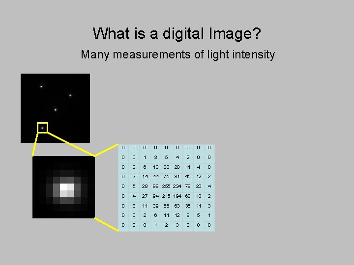
What is a digital Image? Many measurements of light intensity 0 0 0 1 3 5 4 2 0 0 0 2 6 13 20 20 11 4 0 0 3 14 44 75 81 45 12 2 0 5 28 98 255 234 78 20 4 27 94 215 194 68 18 2 0 3 11 39 66 63 35 11 3 0 0 2 6 11 12 8 5 1 0 0 0 1 2 3 2 0 0

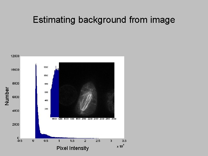
Background correction • Cameras have a non-zero offset • There can also be background fluorescence due to media autofluorescence, etc. • Want to correct for this by background subtraction – Camera dark image – Estimate background from image

Number Estimating background from image Pixel Intensity

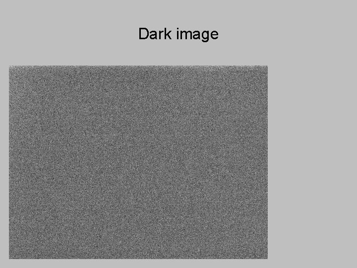
Dark image • Acquired with no light going to the camera – Allows you to measure instrument background – Can detect what’s real background autofluorescence

Dark image

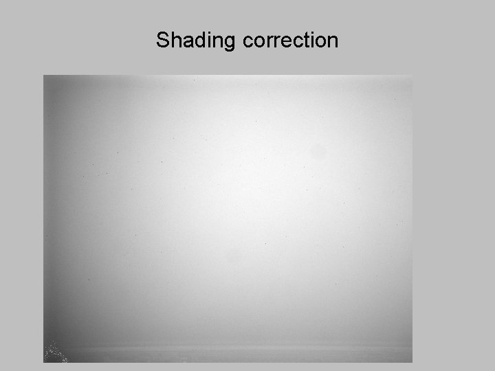
Shading correction • Measure and correct for nonuniformity in illumination and detection • Image a uniform fluorescent sample

Shading correction

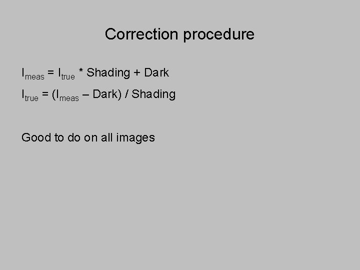
Correction procedure Imeas = Itrue * Shading + Dark Itrue = (Imeas – Dark) / Shading Good to do on all images

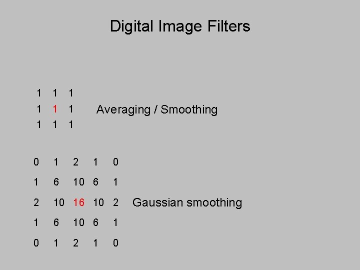
Digital Image Filters 1 1 1 1 1 0 1 2 1 0 1 6 10 6 1 2 10 16 10 2 1 6 10 6 1 0 1 2 0 Averaging / Smoothing 1 Gaussian smoothing

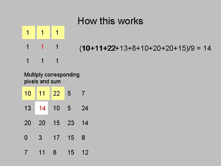
How this works 1 1 1 1 1 (10+11+22+13+8+10+20+20+15)/9 10 +11+22 = 14 Multiply corresponding pixels and sum 10 11 22 5 7 13 814 10 5 24 20 20 15 23 14 0 3 17 15 8 7 11 6 15 12

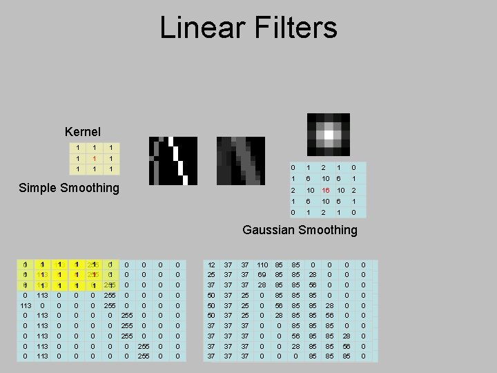
Linear Filters Kernel 1 1 1 1 1 Simple Smoothing 0 1 2 1 0 1 6 10 6 1 2 10 16 10 2 1 6 10 6 1 0 1 2 1 0 Gaussian Smoothing 1 0 0 1 0 113 0 0 0 1 11 0 113 01 1 1 113 0 0 0 113 0 113 0 1 01 01 1 0 0 0 0 1 255 01 0 0 0 1 255 1 0 255 0 0 0 255 0 0 0 0 0 0 0 12 25 37 50 50 50 37 37 37 38 37 37 37 110 37 38 69 69 37 28 25 0 37 0 85 85 85 56 28 0 0 85 85 56 28 0 0 28 56 85 85 0 0 28 56 85 85 0 0 0 0 28 56 85 0 0 0 0 0

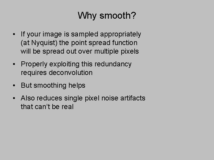
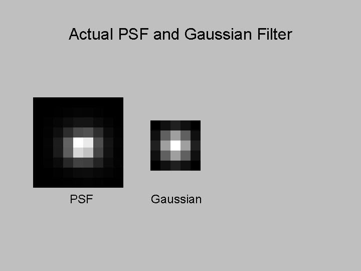
Why smooth? • If your image is sampled appropriately (at Nyquist) the point spread function will be spread out over multiple pixels • Properly exploiting this redundancy requires deconvolution • But smoothing helps • Also reduces single pixel noise artifacts that can’t be real

Actual PSF and Gaussian Filter PSF Gaussian

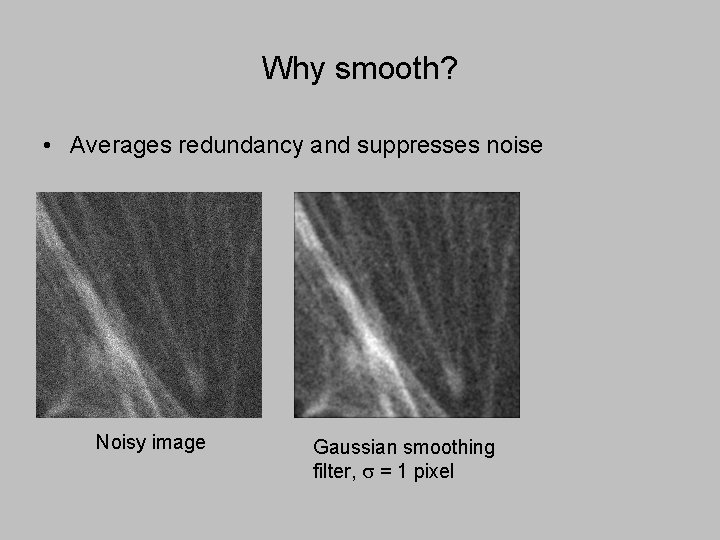
Why smooth? • Averages redundancy and suppresses noise Noisy image Gaussian smoothing filter, s = 1 pixel

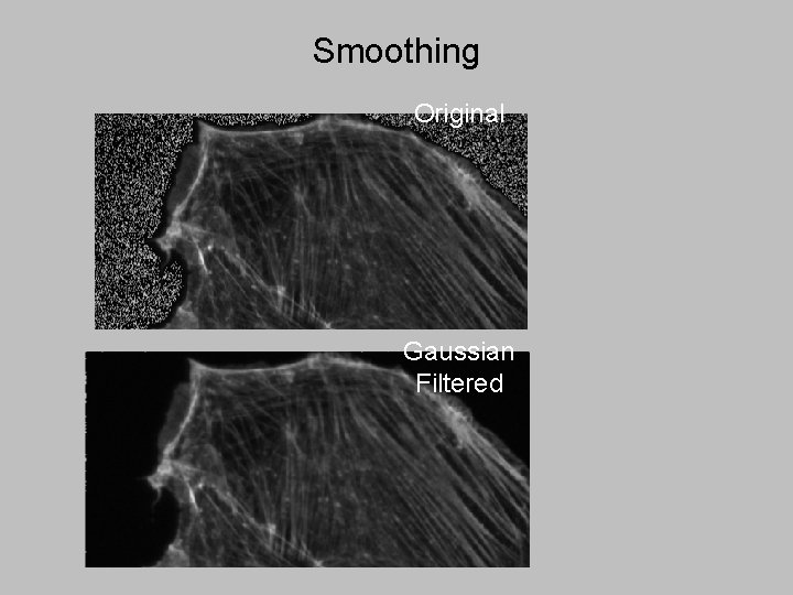
Smoothing Original Gaussian Filtered

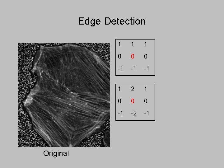
Edge Detection Original 1 1 1 0 0 0 -1 -1 -1 1 2 1 0 0 0 -1 -2 -1

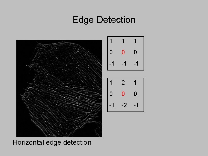
Edge Detection Horizontal edge detection 1 1 1 0 0 0 -1 -1 -1 1 2 1 0 0 0 -1 -2 -1

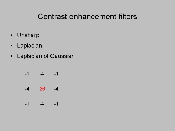
Contrast enhancement filters • Unsharp • Laplacian of Gaussian -1 -4 26 -4 -1

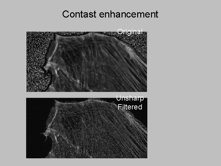
Contast enhancement Original Unsharp Filtered

Nonlinear filters • Can do things like median filtering – replace center pixel by median value within box • Good for smoothing while maintaining edges

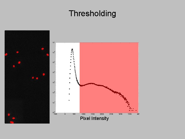
Thresholding Pixel Intensity

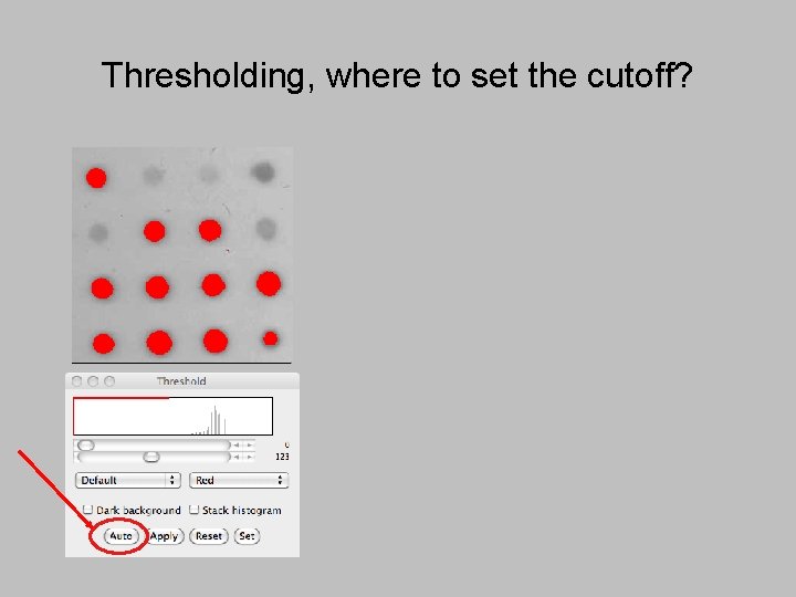
Thresholding, where to set the cutoff?

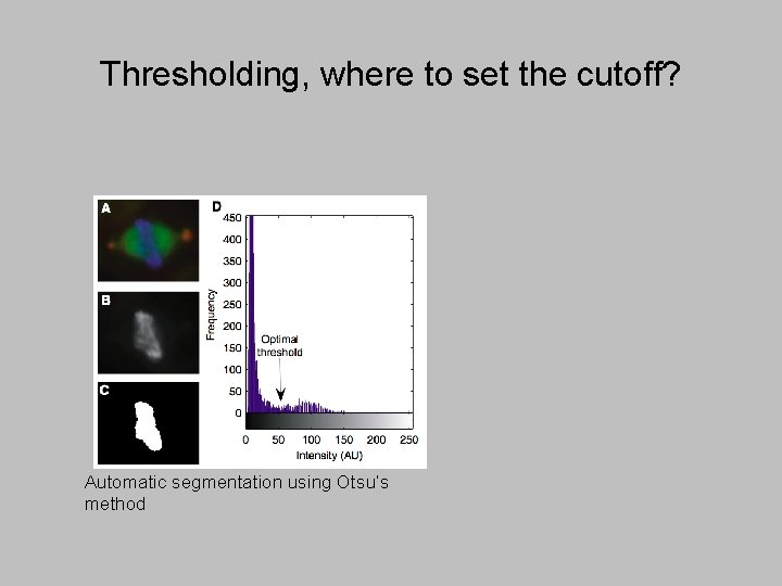
Thresholding, where to set the cutoff? Automatic segmentation using Otsu’s method

One problem with this approach… • It’s biased towards brighter objects • Ideally would use second channel to independently define objects to measure

Binary images • Thresholding gives you a binary image; 1 inside an object, 0 elsewhere • This can be used to identify objects • It can also be manipulated

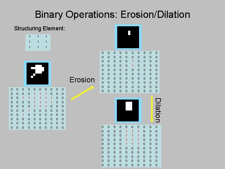
Binary Operations: Erosion/Dilation Structuring Element: 1 1 1 1 1 Erosion 0 0 0 1 0 0 0 0 0 1 1 1 1 0 0 0 0 0 0 0 1 1 0 0 0 0 0 0 0 0 0 0 0 0 0 0 0 0 0 0 0 0 0 0 0 0 0 0 0 0 0 0 0 0 0 0 0 1 1 1 1 0 0 0 0 0 0 0 0 0 0 0 0 Dilation 0 0 0 0 0 0 0 0

Other binary operations • Sequential erosion and dilation – tends to smooth objects • Hole filling • Removing objects at borders

Acknowledgements & Further Reading • Nico Stuurman • Gonzalez, Woods, and Eddins: Digital Image Processing (Using Matlab) • Burger and Burge, Digital Image Processing, An Algorithmic Introduction using Java (Image. J) • Pawley: Handbook of Biological Confocal Microscopy