Digital Image Processing Digital Image ProcessingGonzalez RC Woods

Digital Image Processing 参考书目录： • Digital Image Processing，Gonzalez RC & Woods RE，Prentice Hall，2007 • Pattern Classification & Scene Analysis， Duda RO & Hart PE ，John Wiley & Sons Inc, 1973 • Digital Image Processing Using MATLAB， Gonzalez RC，Woods RE & Eddins SL， Prentice Hall ，2003 • Matlab，the Math. Work Inc.

Chapter 1 Introduction

What is Digital Image Processing? • Vision is the ability to perceive and recognize geometrical objects, patterns, texture, and etc, and to associate them with some functionality or meaning. • Recognizing and associating are two different processes. • The goal of Digital Image Processing is to enable the process of recognition. • The ultimate goal of DIP is to enable a computing machine to recognize at least geometrical sizes, shapes and other objects as in human vision.

What is Digital Image Processing? • DIP is not an electronic equivalent to human vision in any way. • DIP is a branch of Artificial Intelligence (AI). • An attempt to emulate human vision is called weak AI. • To exactly produce a human replica electronically is called strong AI.

Original Image - Lena with noise removal by lowpass filter

Original Image - Lena Binary Lena by Otsu thresholding method Contour Lena by contour following for binary Lena

Original Image - Lena Edge map by Robert operator Enhanced Lena by Histogram Euqalization Edge map by Sobel operator

Applications of Digital Image Processing 1. In Flexible Manufacturing Systems: • • Product Inspection Pick-and-Place Assembly Vehicle Guidance 2. In Biomedical Engineering: • • • Analyzing Chromosome Tomography X-ray Analysis Mammograms Thermograms

Medical product inspection

Image analysis for chromosome deficiency identification in maize

Applications of Digital Image Processing 3. In Military Areas: • • Bomb Disposal Infra-red Night Vision Radar Image Processing Target Identification 4. In Civilian Areas: • • Telecommunications Fire fighting Fingerprint detection (biometrics) Intelligent Vehicle Highway System

Fingerprint Detection System

Applications of Digital Image Processing 5. In Commercial Areas: • • • Bar Code Reader Text Reader Script Reader Desk Top Publishing Multimedia • • • Fingerprint Detection Space Exploration Nuclear Reactor Geographic Studies Archaeology Physics 6. In Scientific Experiments:

A Brief Historic Review 1920 Pictures were transmitted between London and New York via submarine cable 1921 Photographic reproduction techniques were used to print the transmitted pictures 1929 The number of brightness levels (grey levels) was increased from 5 to 15, and the reproduction system improved 1964 Computers were fist used in Jet Propulsion Lab (JPL) to process images from space probes. Now Digital Image processing and pattern classification are used in many areas.

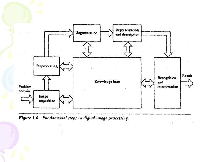
DIGITAL IMAGE PROCESSING SYSTEM OVERVIEW 1. Image Capturing System • • • To sample an analog input and reconstruct a digital version of the image. CCD or video camera Frame grabber and memory Lighting instruments Image is normally degraded by noisy environment, poor light conditions, incorrect camera calibration and quantization error. 2. Image Enhancement System • • To improve the fidelity of the image before feature extraction Brightness, contrast, sharpness, smoothness, distortion, contortion.

DIGITAL IMAGE PROCESSING SYSTEM OVERVIEW 3. Feature Extraction System • Extracts the features of the objects contained in the image • Main features point, lines, edges or regions. • Other features are light intensity, histogram, textures, color. 4. Feature Representation and Description System • Coding of object features into a certain optimal form • Some are symbolic, and some are structural. • To reduce the amount of data processed and stored.

DIGITAL IMAGE PROCESSING SYSTEM OVERVIEW 5. Object Classification System • To compare the current object with some known objects in the image database. • To learn the object if no known objects are found. • Associate a known argument or functionality to the object.

Chapter 2 Digital Image Acquisition The major purpose of this chapter is to describe how sensors produce digital images from the real objects. The 2 D digital image is an array of intensity (亮度) samples reflected from or transmitted through objects: This image is processed by a computer program. Often, a 2 D image represents a projection of a 3 D scene; this is the most common representation used in pattern recognition.

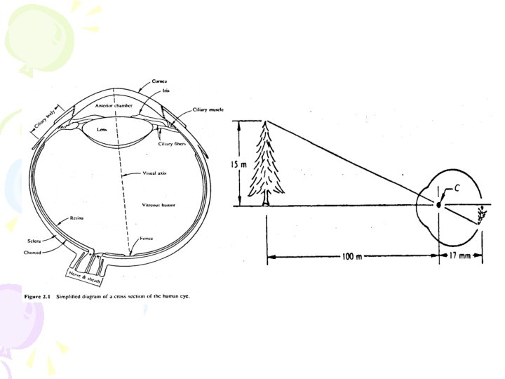
Human Perception and Image Capture Crudely speaking, the human eye is a spherical camera 球形照相 机 with a 20 mm focal length lens at the outside focusing the image on the retina � 网膜 which is opposite the lens and fixed on the inside of the surface of the sphere. The iris 虹膜 controls the amount of light passing through the lens by controlling the size of the pupil 瞳孔. Each eye has one hundred million receptor cells ‑ quite a lot compared to a typical CCD array. The retina is unevenly populated with sensor cells. An area near the center of the retina, called the fovea � 网膜中心 凹, has a very dense concentration of color receptors, called cones ��. Away from the center, the density of cones decreases while the density of black‑white receptors, the rods, increases.

1. Sensing Light Devices can sense and produce different types of electromagnetic radiation 辐射, such as radio waves 无线电波, X‑rays, microwaves 微波, etc. The human eyes are sensitive to radiation (light) with wavelengths ranging from roughly 400 nanometers (blue) to 800 nanometers (red). Visible light X-rays Ultraviolet Blue 紫外线 400 Green Wavelength (nanometers) Red 800 Infrared 红外线

A simple model of common photography: A surface element, illuminated by a single source (the sun or a flash bulb) reflects radiation toward the camera, which senses it via chemicals on film. OBJECT Point source of illumination Surface element Surface normal N Irradiance 发光 Surface reflectance Radiance 光辉 Z CAMERA Optical axis Sensor element

2. Image Devices There are many different devices that produce digital images. They differ in the phenomena sensed as well as in their electromechanical design. (1) CCD Cameras The charge‑coupled device (CCD) is the most flexible and common input device for machine‑vision systems. The CCD camera is very much like a 35 mm film camera commonly used for family photos. The tiny solid state cells convert light energy into electrical charge. The image plane acts as a digital memory that can be read row by a computer input process.

Figure --- A CCD (charge‑coupled device) camera imaging a cylinder; discrete cells convert light energy into electrical charges, which are represented as small numbers when input to a computer. Read row or pixel 3 D Scene Lens Image Alternative analog TV signal plane Pixel To Frame Buffer To TV

Pixel Digital image is in discrete form

Pixel Digital image is in discrete form

Pixel G y ra Digital image le ve 6 19 l 92

Figure --- An entire computer system with both camera input and graphics output. Camera CCD array Lens 3 D Scene A/D Machine vision algorithm Graphic display Frame buffer Display processor It is a typical system for an industrial‑vision 业 task or medical‑imaging 医学 task. It is also typical for multimedia 多媒体 computers. The camera provides analog image 模拟图像. A/D 模数转化 converts the analog image to digital image. The Frame buffer is a high speed image store for digital image. The digital image in the frame buffer is available for display and for processing by computer algorithms.

Picture Functions and Digital Images We now discuss some concepts and notation important for both theory and programming of image‑processing operations.

(1) Types of Images Definition-1: An analog image 模�� 像 is a 2 D image F(x, y) which - has infinite precision in spatial parameters x and y, and - infinite precision in intensity at each spatial point (x, y). yi=Real number y f(xi, yi)=Real number xi=Real number x

Definition-2: A digital image 数字图像 is a 2 D image I[r, c] represented by a discrete 2 D array of intensity samples, each of which is represented using a limited precision. yi=Integer y f(xi, yi)=Integer xi=Integer x It is common to record intensity as an 8‑bit (1‑byte) number which allows values of 0 to 255. 256 different levels is usually all the precision available - from the sensor and - also is usually enough to satisfy the consumer.

Different coordinate systems used for images • raster oriented 光�� 向 uses row and column coordinates starting at [0, 0] from the top left c I[0, 0] I[M-1, N-1] r I[M-1, 0] y • Cartesian 笛卡尔 coordinate frame with [0, 0] at the lower left F[M-1, N-1] F[0, 0] x

• Cartesian coordinate frame with [0, 0] at the image center y [W/2, H/2] x [0, 0] [-W/2, -H/2] • Relationship of pixel center point [x, y] to area element sampled in array element I[i, j] [x 0+i x, y 0+j y] F[i, j] [x 0, y 0] F[i+1, j]

Some Definitions Definition-3: A picture function is a mathematical representation f(x, y) of a picture as a function of two spatial variables x and y are real values defining points of the picture. f(x, y) is usually also a real value defining the intensity of the picture at point (x, y). f(x, y)=89 f(x, y)=0 Definition-4: A gray‑scale image 单色灰度图像 is a monochrome digital image f(x, y) with one intensity value per pixel. f(x, y)=218

Definition-5: A multispectral image 彩色图像 is a 2 D image M[x, y], which has a vector of values at each spatial point or pixel. If the image is actually a color image, then the vector has 3 elements.

Definition-5 -M: Colour vision depends on three types of cone cells, each with its own relative luminance efficiency function which measures the sensitivity of the respective type of cone cells to different frequencies of light. ( ) 450 nm (blue) 550 nm (Green) 640 nm (yellow-green) From these curves, we can see that the human vision system is biased towards the colour green (note the significant overlap between S 1 and S 2).

( ) 450 nm (blue) 550 nm (Green) 640 nm (yellow-green) To mimic the way we see colour, all colour image formats are based on three components, one for each of the three primary colours: Red, Green and Blue (RGB) or some linear combinations of them. There are 100 million rod cells on a human retina (roughly equivalent to 10, 000 dpi) versus 6. 5 million cone cells 视锥细胞.

Definition-6: A binary image 二值图像 is a digital image with all pixel values 0 or 1. f(x, y)=1 y f(x, y)=0 x A B图像

Definition-7: A labeled image 分类图像 is a digital image L[r, c] whose pixel values are symbols. The symbol value of a pixel denotes the outcome of some decision made for that pixel. Original image Labeled image Boundaries of the extracted face region

Original image (tiger) Labeled image

(2) Image Spatial Measurement and Quantization Definition-8: The nominal resolution 标称分辨度 of a CCD sensor is the size of the scene element that images to a single pixel on the image plane. Each pixel of a digital image represents a sample of some elemental region of the real image. Size of scene element Image Plane pixel 3 D Scene pixel Lens

If the pixel is projected from the image plane back out to the source material in the scene, then the size of that scene element is the nominal resolution � 称分辨度 of the sensor. Image Plane pixel 3 D Scene Lens

For example, if a 10 inch square sheet of paper is imaged to form a 500 digital image, then the nominal resolution of the sensor is 0. 02 inches (10/500 = 0. 02). 10 10 inch 2 500

Definition-9: The term resolution refers to the precision of the sensor in making measurements, but is formally defined in different ways. If defined in real world terms, it may just be the nominal resolution, as in “the resolution of this scanner is one meter on the ground” Or it may be in the number of line pairs per millimeter that can be resolved or distinguished in the sensed image. Definition-10: The field of view 视野of a sensor (FOV) is the size of the scene that it can sense, for example 10 inches by 10 inches.

(a) Digital image with 127 rows of 176 columns; (b) (63 88) created by averaging each 2 2 neighborhood of (a) and replicating the average to produce a 2 2 average block; (c) (31 44) created in same manner from (b); and (d) (15 22) created in same manner from (c). Effective nominal resolutions are (127 176), (63 88), (31 44), and (15 22) respectively.

Image Quantization � 像量化 A quantizer is an Analog-to-Digital device which converts a continuous input signal u to one of a set of discrete levels called reconstruction levels rk. Suppose the u lies in the range: umin u umax and we wish to quantize u into L levels. Then we define L+1 transition levels tk: t 0 = umin<t 1<……<t. L-1<t. L = umax The quantization step involves mapping u to its quantized value, u*, using the rule: Define {tk, k = 0, …, L} as a set of increasing transition or decision levels with t 0 and t. L as the minimum and maximum values, respectively, of u.

A graphical representation (staircase map) of the quantization function is as below: r. L u Quantizer u* u* rk t 0 tk t. L u r 0 Usually, L = 2 B (B-bit representation). D = t. L –t 0 = umax - umin is called the dynamic range. Error of quantization clearly depends on L and D, as well as on the choice of reconstruction levels and transition levels.

Lloyd-Max quantizer - LM量化器 Let us model the intensity of the image u as a random variable with continuous probability density function (p. d. f. ) pu(u). We would like to construct a quantizer (with decision levels tk and reconstruction levels rk), which minimizes the mean square error, i. e. where u* is the quantization of u, i. e. (1) To minimize this measure of quantization error, we differentiate with respect to tk and rk, and set them to zero.

Mathematically, the decision and reconstruction levels are solutions to the following set of nonlinear equations: (2) Similarly, (3) In general, Eqs. (2) and (3) do not yield closed-form solutions, and they need to be solved by numerical techniques. Solving the above equations yields the optimal Lloyd-Max quantizer 最佳LM量化器.

Special case – Uniform Distribution From Eq. (3), we can obtain (4)

Combining Eq. (2) and (4), we get which gives where the constant q is called the quantization interval. • Finally, we obtain For this uniform quantizer, the quantization error is

It is easy to see that Thus, the quantization error is small when the quantization interval q is small.

It is usual to compare errors with signal variance: when the signal is smooth, then even relatively small errors would become noticeable whereas for signals with large fluctuations, noise become less significant. Let u 2 be the variance of the signal u. For a uniformly distributed signal, its mean is E(u)=(t. L +t 1)/2, and we have

Instead of talking about L levels, it is common to talk about bit representation, i. e. let L = 2 B, where B is the number of bits, then the signal-to-noise ratio is defined as i. e. every bit improves the SNR by 6 decibels. Thus an 8 -bit image has a signal to noise ratio of 48 d. B, which is very good for practical applications. in practice, there are many sources of noise in addition to quantization noise, and the concept of signal to noise ratio can be similarly defined to measure their effects.

Some Problems in Image Quantization (a) 10 10 array of black (brightness 0) and white (brightness 8) tiles; (0+0+0+8)/4 = 2 (b) Intensities recorded in a 5 5 image of precisely the brightness field at the above, where each pixel senses the average brightness of a 2 2 neighborhood of tiles;

(0+0+0+8)/4 =2

Note that the quantized brightness values depend on both the actual pixel size and position relative to the brightness field; (c) Image sensed by shifted camera one tile down and one tile to the right. (8+0+0+0)/4 = 2 (d) Intensities recorded from the shifted camera in the same manner as in (b). 0 0 0 0 8 0 8 8 0

Interpretation of the actual scene features will be problematic with either image (b) or (d). Note that the quantized brightness values depend on both the actual pixel size and position relative to the brightness field. Different digital images (b) (d)

Effects of Quantization The resolution depends on the spatial quantization (the number of samples per inch) Colour image Gray-scale image 512 X 256 Gray-scale image 256 X 128

Effects of Quantization The resolution depends on the spatial quantization (the number of samples per inch) Gray-scale image 128 X 64 Gray-scale image 64 X 32 Gray-scale image 32 X 16

Effects of Quantization The quality of the image depends on the intensity quantization (the number of gray levels) 8 -Bit image (256 levels) 7 -Bit image (128 levels)

6 -Bit (64 levels) 5 -Bit (32 levels) 4 -Bit (16 levels) 3 -Bit (8 levels)

Effects of Quantization The quality of the image depends on the intensity quantization (the number of gray levels) 2 -Bit image (4 levels) 1 -Bit image (2 levels)

Effects of Quantization

5. Digital Image Formats* Standard formats have been developed so that different hardware and software can share data. Read file Application (Web search) Write file Application (scanner) Image file Device, database, or channel Application (image proc) Application (doc proc) Image file Standard format Application (OCR) Application …… Many devices or application programs create, consume, or convert image data. Standard format image files are needed to do this productively for a family of devices and programs.

Commonly Used Formats: Raw image (non-standard image) Run-coded binary images Portable bit map Family (PBM/PGM, PPM) Graphics interchange Format (GIF) Tag image file format (TIFF/TIF) JPEG (JFIF/JFI/JPG) format for still photos Post. Script family (BDF/PDL/EPS) MPEG (MPG/MPEG-1/MPEG-2) format for video

Non-Standard Image (Raw Image): A raw image may be just a stream of bytes encoding the image pixels in row‑by‑row order, called raster order, perhaps with line‑feeds separating rows. Standard Image: Most recently developed standard formats contain a header with non‑image information necessary to label the data and to decode it. Image File Header --- • A file header is needed to make an image file self‑describing so that image‑processing tools can work with them. • The header should contain the image dimensions, type, date of creation, and some kind of title. • It may also contain a color table or coding table to be used to interpret pixel values.

Image Data --Some formats can handle only limited types of images. Pixel size and image size limits typically differ between different file formats. Several formats can handle a sequence of frames. Multimedia formats are evolving and include image data along with text, graphics, music, etc. Data Compression --Many formats provide for compression of the image data so that all pixel values are not directly encoded. Image compression can reduce the size of an image to 30 percent or even 3 percent of its raw size. Compression can be lossless or lossy. With lossless compression, the original image can be recovered exactly. With lossy compression, the pixel representations cannot be recovered exactly.

Commonly Used Formats: 1. Run‑Coded Binary Images Run‑coding is an efficient coding scheme for binary or labeled images: not only does it reduce memory space, but it can also speed up image operations. Example: Image Row r 00001111100000011100000001111100000 Run‑code A 8(0)5(1)12(0)3(1)7(0)9(1)5(0) Run‑coding is often used for compression within standard file formats.

2. PGM: Portable Gray Map One of the simplest file formats for storing and exchanging image data is the PBM or Portable Bit Map family of formats (PBM/PGM, PPNI). The image header and pixel information are encoded in ASCII. P 2 # sample small picture 8 rows of 16 columns, max gray value of 192 # making an image of the word "Hi". 16 8 192 Printed picture Image made using a lossy compression algorithm

3. GIF Image File Format The Graphics Interchange Format (GIF) originated from Compu. Serve, Inc. It has been used to encode a huge number of images on the World Wide Web or in current databases. GIF files are relatively easy to work with, but cannot be used for high‑precision color, since only 8‑bits are used to encode color. 4. TIFF Image File Format TIFF or TIF is very general and very complex. It is used on all popular platforms and is often the format used by scanners. It supports multiple images with 1 to 24 bits of color per pixel. TIFF or TIF is available for either lossy or lossless compression.

5. JPEG Format for Still Photos JPEG (JFIF/JFI/JPG) is a more recent standard from the Joint Photographic Experts Group. The major purpose is to provide for practical compression of high‑quality color still images. An image can have up to 64 K pixels of 24 bits each. 6. Post. Script The family of formats BDF/PDL/EPS store image data using printable ASCII characters and are often used with X 11 graphics displays and printers. PDL is a page description language EPS is encapsulated postscript (originally from Adobe), which is commonly used to contain graphics or images to be inserted into a larger document.

7. MPEG Format for Video MPEG (MPG/MPEG‑ 1/MPEG‑ 2) is a stream‑oriented encoding scheme for video, audio, text, and graphics. MPEG stands for Motion Picture Experts Group, an international group of representatives from industry and governments. MPEG‑ 1 is primarily designed for multimedia systems and provides for a data rate of 0. 25 Mbits per second of compressed audio and 1. 25 Mbits of compressed video. These rates are suitable for multimedia for popular personal computers, but are too low for high‑quality TV. MPEG‑ 2 standard provides for up to 15 Mbits per second data rates to handle high definition TV rates. The compression scheme takes advantage of both spatial redundancy, as used in JPEG, and temporal redundancy and generally provides a useful compression ratio of 25 to 1, with 200 to 1 ratios possible.

Comparison of Formats Table File sizes (in bytes) for the same image encoded in different formats: 8 x 16 gray‑level "hi" image 347 x 489 color "cars" image. Image File Format PGM GIF TIF PS HIPS JPG (lossless) JPG (lossy) No. Bytes “Hi” No. Bytes “Cars” 595 192 918 1, 591 700 684 619 509, 123 138, 267 171, 430 345, 387 160, 783 49, 160 29, 500