Indifference curves Introduction In microeconomic theory an indifference

Indifference curves

Introduction • In microeconomic theory, an indifference curve is a graph showing different bundles of goods, each measured as to quantity, between which a consumer is indifferent. • That is, at each point on the curve, the consumer has no preference for one bundle over another. In other words, they are all equally preferred.

• One can equivalently refer to each point on the indifference curve as rendering the same level of utility (satisfaction) for the consumer. • Utility is then a device to represent preferences rather than something from which preferences come.

• In economics, utility is a measure of relative satisfaction. • Given this measure, one may speak meaningfully of increasing or decreasing utility, and thereby explain economic behavior in terms of attempts to increase one's utility. • Utility is often modeled to be affected by consumption of various goods and services, possession of wealth and spending of leisure time

• The main use of indifference curves is in the representation of potentially observable demand patterns for individual consumers over commodity bundles

properties of indifference curves • 1. defined only in the positive (+) quadrant of commodity-bundle quantities. • 2. negatively sloped. That is, as quantity consumed of one good (X) increases, total satisfaction would increase if not offset by a decrease in the quantity consumed of the other good (Y). Equivalently, satiation, such that more of either good (or both) is equally preferred to no increase, is excluded. (If utility U = f(x, y), U, in the third dimension, does not have a local maximum for any x and y values. )

• 3. complete, such that all points on an indifference curve are ranked equally preferred and ranked either more or less preferred than every other point not on the curve. So, with (2), no two curves can intersect (otherwise non-satiation would be violated). • 4. transitive with respect to points on distinct indifference curves.

• That is, if each point on I 2 is (strictly) preferred to each point on I 1, and each point on I 3 is preferred to each point on I 2, each point on I 3 is preferred to each point on I 1. • A negative slope and transitivity exclude indifference curves crossing, since straight lines from the origin on both sides of where they crossed would give opposite and intransitive preference rankings.

• 5. (strictly) convex (sagging from below). • With (2), convex preferences implies a bulge toward the origin of the indifference curve. • As a consumer decreases consumption of one good in successive units, successively larger doses of the other good are required to keep satisfaction unchanged, the substitution effect.

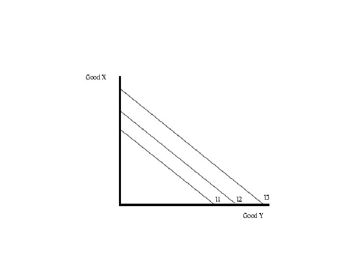
Example Indifference Curves Below is an example of an indifference map having three indifference curves:

• The consumer would rather be on I 3 than I 2, and would rather be on I 2 than I 1, but does not care where they are on each indifference curve. • The slope of an indifference curve, known by economists as the marginal rate of substitution, shows the rate at which consumers are willing to give up one good in exchange for more of the other good

• For most goods the marginal rate of substitution is not constant so their indifference curves are curved. • The curves are convex to the origin indicating a diminishing marginal rate of substitution.

• If the goods are perfect substitutes then the indifference curves will be parallel lines since the consumer would be willing to trade at a fixed ratio. • The marginal rate of substitution is constant.

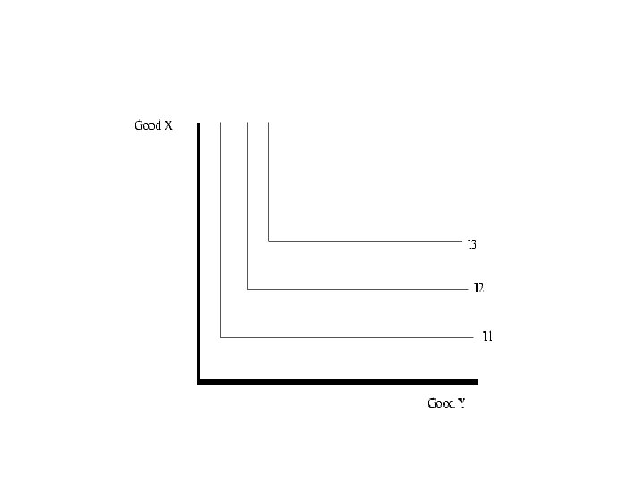
• If the goods are perfect complements then the indifference curves will be L-shaped. An example would be something like if you had a cookie recipe that called for 3 cups flour to 1 cup sugar. No matter how much extra flour you had, you still could not make more cookie dough without more sugar. Another example of perfect complements is a left shoe and a right shoe. The consumer is no better off having several right shoes if she has only one left shoe. Additional right shoes have zero marginal utility without more left shoes. The marginal rate of substitution is either zero or infinite.

The Price Consumption Curve • shows how much of a commodity (x) is bought at a certain price of (x). – up and down of curve is not interesting for (x), what matters are movements to the left & right – if from left to right, then an increasing amount of commodity (x) is in every bundle • “More is required at a lower price” is NOT an assumption – Curve might move from right to left! • The Question therefore is; under which conditions will a falling price lead to an increase in demand? Price Consumption Curve, increase in consumption of (x)

PPC.