Idiots guide to General Linear Model f MRI

Idiot's guide to. . . General Linear Model & f. MRI • f. MRI model, Linear Time Series, Design Matrices, Parameter estimation, *&%@! Elliot Freeman, ICN.

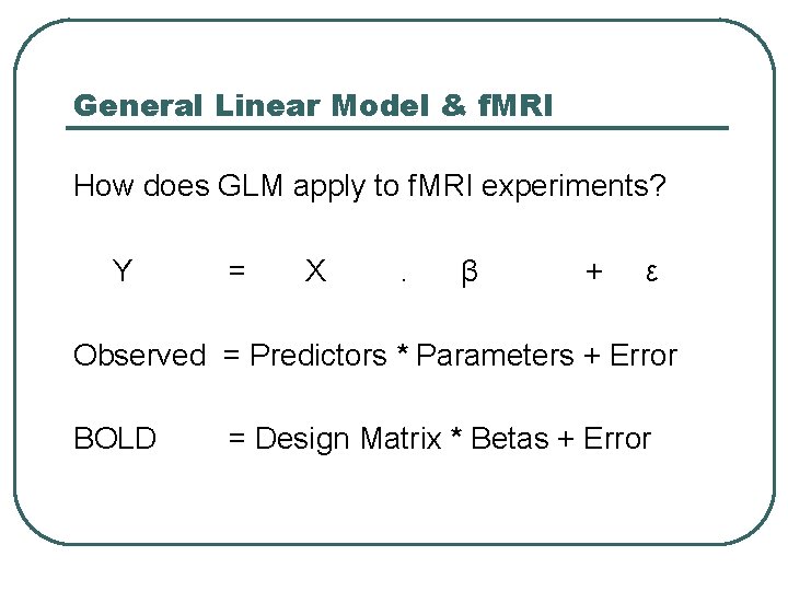
General Linear Model & f. MRI How does GLM apply to f. MRI experiments? Y = X . β + ε Observed = Predictors * Parameters + Error BOLD = Design Matrix * Betas + Error

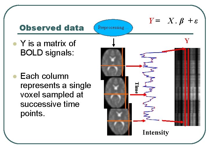
Observed data Y is a matrix of BOLD signals: Each column represents a single voxel sampled at successive time points. Preprocessing. . . X. β +ε Y Time Y= Intensity

Univariate analysis Each voxel considered as independent observation Analysis of individual voxels over time, not groups over space SPM would still work on an Amoeba! Y= X. β +ε

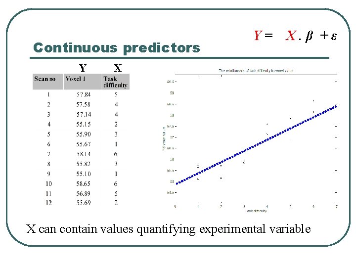
Continuous predictors Y Y= X. β +ε X • X can contain values quantifying experimental variable

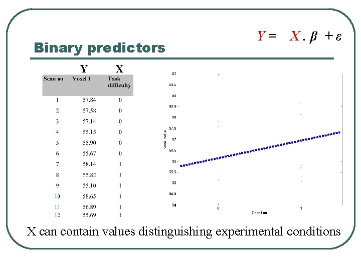
Binary predictors Y Y= X. β +ε X • X can contain values distinguishing experimental conditions

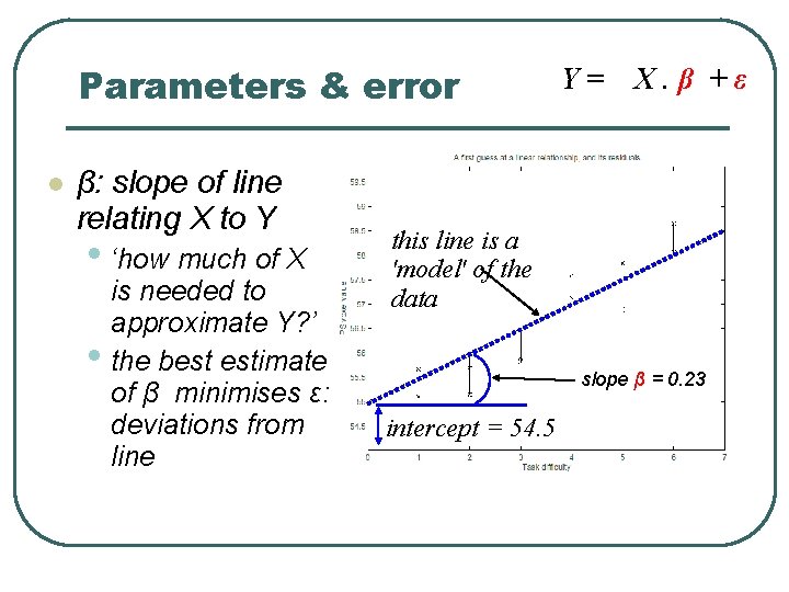
Parameters & error β: slope of line relating X to Y • ‘how much of X • is needed to approximate Y? ’ the best estimate of β minimises ε: deviations from line Y= X. β +ε this line is a 'model' of the data slope β = 0. 23 intercept = 54. 5

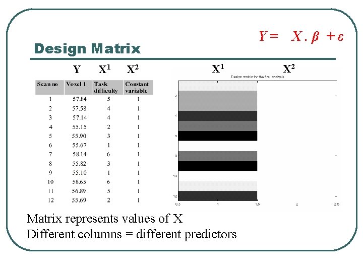
Y= Design Matrix Y X 1 X 2 X 1 • Matrix represents values of X Different columns = different predictors X. β +ε X 2

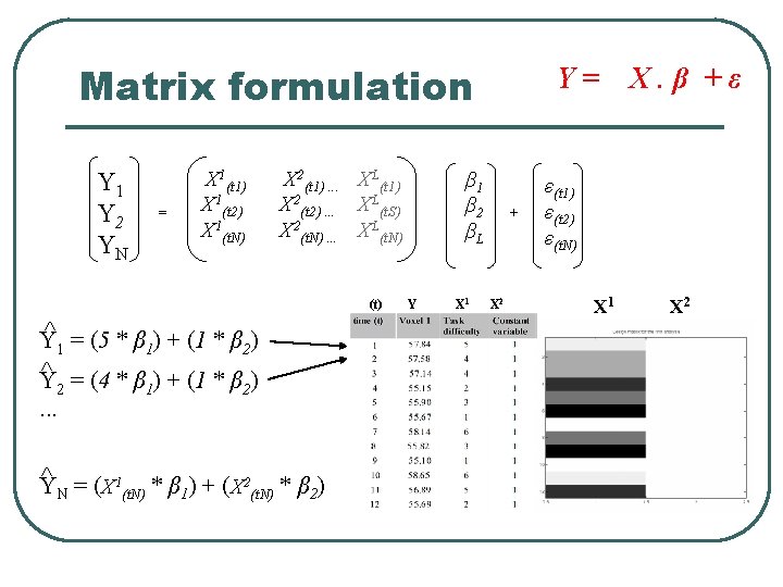
Matrix formulation Y 1 Y 2 YN = X 1(t 1) X 1(t 2) X 1(t. N) X 2(t 1). . . XL(t 1) X 2(t 2). . . XL(t. S) X 2(t. N). . . XL(t. N) (t) ^ = (5 * β ) + (1 * β ) Y 1 1 2 ^ = (4 * β ) + (1 * β ) Y 2 1 2. . . ^ = (X 1 * β ) + (X 2 * β ) Y (t. N) N 1 2 Y= β 1 β 2 βL Y X 1 + X 2 X. β +ε ε(t 1) ε(t 2) ε(t. N) X 1 X 2

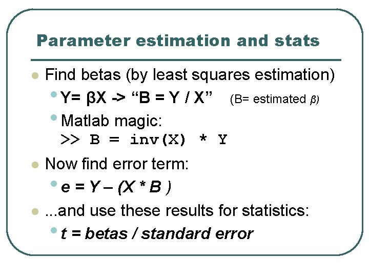
Parameter estimation and stats Find betas (by least squares estimation) • Y= βX -> “B = Y / X” (B= estimated β) • Matlab magic: >> B = inv(X) * Y Now find error term: • e = Y – (X * B ) . . . and use these results for statistics: • t = betas / standard error

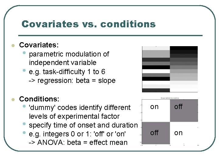
Covariates vs. conditions Covariates: • parametric modulation of independent variable • e. g. task-difficulty 1 to 6 -> regression: beta = slope Conditions: • 'dummy' codes identify different levels of experimental factor • specify time of onset and duration • e. g. integers 0 or 1: 'off' or 'on' -> ANOVA: beta = effect mean on off on

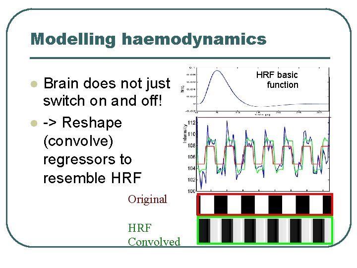
Modelling haemodynamics Brain does not just switch on and off! -> Reshape (convolve) regressors to resemble HRF Original HRF Convolved HRF basic function

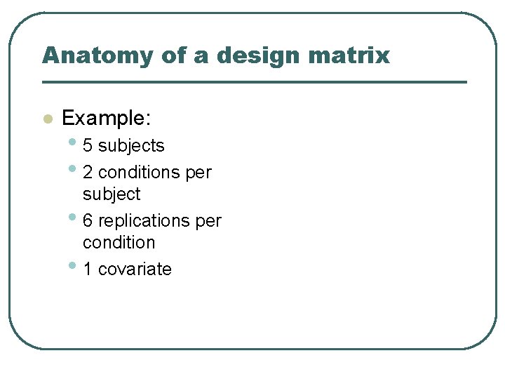
Anatomy of a design matrix Example: • 5 subjects • 2 conditions per • • subject 6 replications per condition 1 covariate

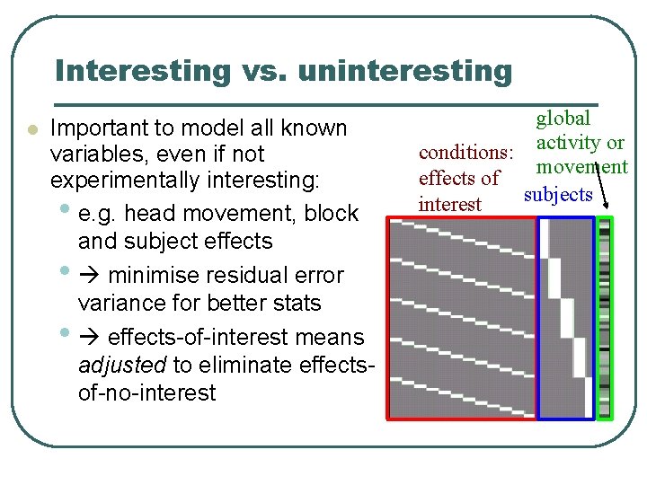
Interesting vs. uninteresting Important to model all known variables, even if not experimentally interesting: • e. g. head movement, block and subject effects • minimise residual error variance for better stats • effects-of-interest means adjusted to eliminate effectsof-no-interest global conditions: activity or movement effects of subjects interest

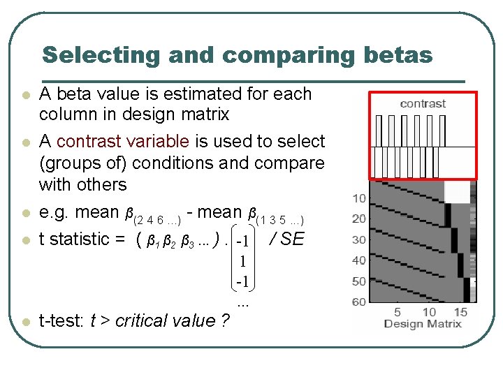
Selecting and comparing betas A beta value is estimated for each column in design matrix A contrast variable is used to select (groups of) conditions and compare with others e. g. mean β(2 4 6. . . ) - mean β(1 3 5. . . ) t statistic = ( β 1 β 2 β 3. . . ). -1 / SE t-test: t > critical value ? 1 -1. . .

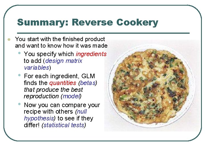
Summary: Reverse Cookery You start with the finished product and want to know how it was made • You specify which ingredients to add (design matrix variables) • For each ingredient, GLM finds the quantities (betas) that produce the best reproduction (model) • Now you can compare your recipe with others (null hypothesis) to see if they differ! (statistical tests)

How dumb was that? Sources: http: //www. fil. ion. ucl. ac. uk/spm/doc/papers/SPM_3/welcome. html http: //www. fil. ion. ucl. ac. uk/spm/doc/books/hbf 2/pdfs/Ch 7. pdf http: //www. mrc-cbu. cam. ac. uk/Imaging/Common/spmstats. shtml