General Linear Model General Linear Model regressors Y

General Linear Model

General Linear Model regressors Y 1 Y 2 X 11 … X 1 l … X 1 L X 21 … X 2 l … X 2 L β 1 β 2 ε 1 ε 2 . . . XJ 1 … XJl … XJL βL = YJ time points Y Observed data = + εJ time points regressors X Design Matrix * β Parameters + ε Residuals/Error

Design Matrix rest task 0 0 0 0 1 1 1 1 Conditions On Off On Use ‘dummy codes’ to label different levels of an experimental factor (eg. On = 1, Off = 0). time

Design Matrix 5 4 4 2 3 1 6 5 2 Covariates Parametric variation of a single variable (eg. Task difficulty = 1 -6) or measured values of a variable (eg. Movement).

Design Matrix 1 1 1 1. . . Constant Variable Models the baseline activity (eg. Always = 1)

Design Matrix Time Regressors The design matrix should include everything that might explain the data.

General Linear Model regressors Y 1 Y 2 X 11 … X 1 l … X 1 L X 21 … X 2 l … X 2 L β 1 β 2 ε 1 ε 2 . . . XJ 1 … XJl … XJL βL = YJ time points Y Observed data = + εJ time points regressors X Design Matrix * β Parameters + ε Residuals/Error

Error • Independent and identically distributed iid

Ordinary Least Squares 35 Residual sum of square: The sum of the square difference between actual value and fitted value. 30 25 20 e 15 10 5 0 0 5 10 15

Ordinary Least Squares 35 N åe t =1 30 2 t = minimum 25 20 15 e 10 5 0 0 -5 5 10 15

Ordinary Least Squares Y = Xβ+e e = Y-Xβ XTe=0 => XT(Y-Xβ)=0 => XTY-XTXβ=0 => XTXβ=XTY => β=(XTX)-1 XTY y Xβ x 1 β 1 x 2 β 2 e

f. MRI Y = Observed data X Design Matrix * β + ε Parameters Residuals/Error 12

Problems with the model

The Convolution Model Expected BOLD HRF Impulses =

Convolve stimulus function with a canonical hemodynamic response function (HRF): HRF Original Convolved HRF

Physiological Problems

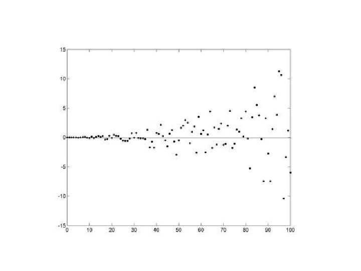
Noise Low-frequency noise Solution: High pass filtering

discrete cosine transform (DCT) set blue black green red = data = mean + low-frequency drift = predicted response, taking into account low-frequency drift = predicted response, NOT taking into account low-frequency drift

Assumptions of GLM using OLS All About Error

Unbiasedness Expected value of beta = beta

Normality

Sphericity

Homoscedasticity

not

Independence

Autoregressive Model y = Xβ + e over time et = aet-1 + ε autocovariance function a should = 0

Thanks to… • Dr. Guillaume Flandin

References • http: //www. fil. ion. ucl. ac. uk/spm/doc/books/hbf 2/pdfs/Ch 7. pdf • http: //www. fil. ion. ucl. ac. uk/spm/course/slides 10 vancouver/02_General_Linear_Model. pdf • Previous Mf. D presentations