The General Linear Model The Simple Linear Model

The General Linear Model

The Simple Linear Model Linear Regression

Suppose that we have two variables 1. Y – the dependent variable (response variable) 2. X – the independent variable (explanatory variable, factor)

X , the independent variable may or may not be a random variable. Sometimes it is randomly observed. Sometimes specific values of X are selected

The dependent variable, Y, is assumed to be a random variable. The distribution of Y is dependent on X The object is to determine that distribution using statistical techniques. (Estimation and Hypothesis Testing)

These decisions will be based on data collected on both variable Y (the dependent variable) and X (the independent variable). Let (x 1, y 1), (x 2, y 2), … , (xn, yn) denote n pairs of values measured on the independent variable (X) and the dependent variable (Y) The scatterplot: The graphical plot of the points: (x 1, y 1), (x 2, y 2), … , (xn, yn)

Assume that we have collected data on two variables X and Y. Let (x 1, y 1) (x 2, y 2) (x 3, y 3) … (xn, yn) denote the pairs of measurements on the on two variables X and Y for n cases in a sample (or population)

The assumption will be made that y 1, y 2, y 3 …, yn are 1. 2. 3. 4. independent random variables. Normally distributed. Have the common variance, s. The mean of yi is mi = a + bxi Data that satisfies the assumptions above is to come from the Simple Linear Model

Each yi is assumed to be randomly generated from a normal distribution with mean mi = a + bxi and standard deviation s. yi s a + bxi xi

• When data is correlated it falls roughly about a straight line.

The density of yi is: The joint density of y 1 , y 2 , …, yn is:

Estimation of the parameters the intercept a the slope b the standard deviation s (or variance s 2)

The Least Squares Line Fitting the best straight line to “linear” data

Let Y=a +b. X denote an arbitrary equation of a straight line. a and b are known values. This equation can be used to predict for each value of X, the value of Y. For example, if X = xi (as for the ith case) then the predicted value of Y is:

Define the residual for each case in the sample to be: The residual sum of squares (RSS) is defined as: The residual sum of squares (RSS) is a measure of the “goodness of fit of the line Y = a + b. X to the data

One choice of a and b will result in the residual sum of squares attaining a minimum. If this is the case than the line: Y = a + b. X is called the Least Squares Line

To find the Least Squares estimates, a and b, we need to solve the equations: and

Note: or and

Note: or

Hence the optimal values of a and b satisfy the equations: and From the first equation we have: The second equation becomes:

Solving the second equation for b: and where and

Note: and Proof

Summary: Slope and intercept of the least squares Line and

Maximum Likelihood Estimation of the parameters the intercept a the slope b the standard deviation s

Recall The joint density of y 1 , y 2 , …, yn is: = the Likelihood function

the log Likelihood function To find the maximum Likelihood estimates of a, b and s we need to solve the equations:

becomes These are the same equations for the least squares line which have solution:

The third equation: becomes

Summary: Maximum Likelihood Estimates and

A computing formula for the estimate of s 2 and Hence

Now Hence

It also can be shown that Thus , the maximum likelihood estimator of s 2, is a biased estimator of s 2. This estimator can be easily converted into an unbiased estimator of s 2 by multiply by the ratio n/(n – 2)

Estimators in Linear Regression and

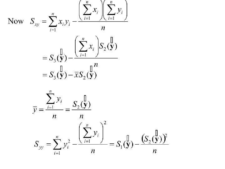
The major computation is :

Computing Formulae:

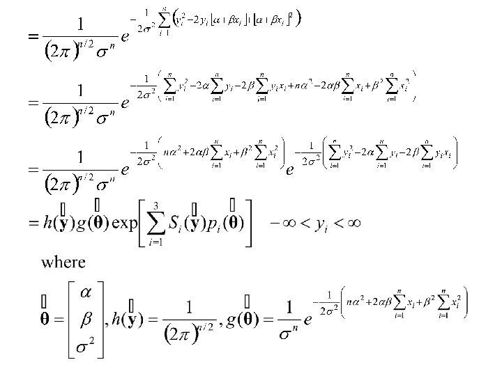
Application Of Statistical Theory to simple Linear Regression We will now use statistical theory to prove optimal properties of the estimators. Recall, the joint density of y 1 , y 2 , …, yn is:

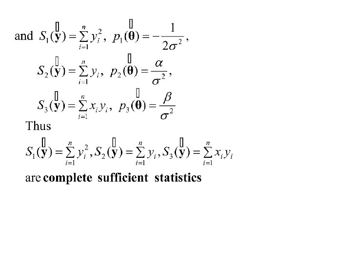
Also and Thus all three estimators are functions of the set of complete sufficient statistics. If they are also unbiased then they are Uniform Minimum Variance Unbiased (UMVU) estimators (using the Lehmann-Scheffe theorem)

We have already shown that s 2 is an unbiased estimator of s 2. We need only show that: and are unbiased estimators of b and a.

Thus are unbiased estimators of b and a.

Also Thus

The General Linear Model

Consider the random variable Y with 1. E[Y] = b 1 X 1+ b 2 X 2 +. . . + bp. Xp (alternatively E[Y] = b 0+ b 1 X 1+. . . + bp. Xp, intercept included) and 2. var(Y) = s 2 • where b 1, b 2 , . . . , bp are unknown parameters • and X 1 , X 2 , . . . , Xp are nonrandom variables. • Assume further that Y is normally distributed.

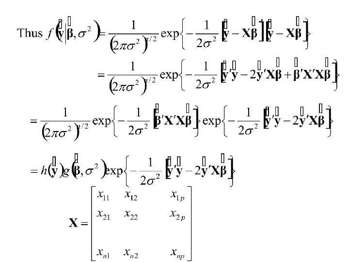
Thus the density of Y is: f(Y|b 1, b 2 , . . . , bp, s 2) = f(Y| , s 2)

Now suppose that n independent observations of Y, (y 1, y 2, . . . , yn) are made corresponding to n sets of values of (X 1 , X 2 , . . . , Xp) (x 11 , x 12 , . . . , x 1 p), (x 21 , x 22 , . . . , x 2 p), . . . (xn 1 , xn 2 , . . . , xnp). Then the joint density of y = (y 1, y 2, . . . yn) is: f(y 1, y 2, . . . , yn|b 1, b 2 , . . . , bp, s 2) =

Thus is a member of the exponential family of distributions And is a Minimal Complete set of Sufficient Statistics.

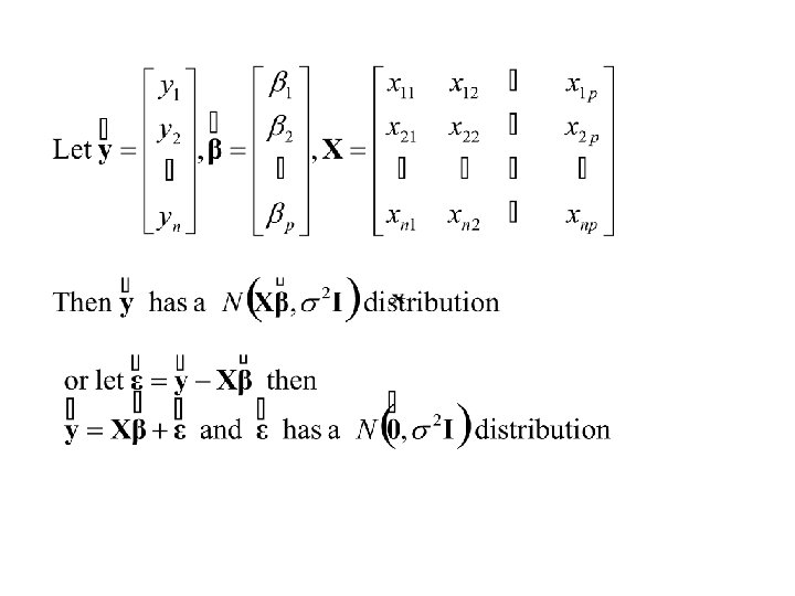
Matrix-vector formulation The General Linear Model

The General Linear Model

Geometrical interpretation of the General Linear Model

Geometical interpretation of the General Linear Model

Estimation The General Linear Model

Least squares estimates of b Let

The Equations for the Least squares estimates

Written out in full These equations are called the Normal Equations

Matrix development of the Normal Equations Now The Normal Equations

Summary (the Least Squares Estimates) The Least Squares estimates satisfy The Normal Equations

Note: Some matrix properties Rank rank(AB) = min(rank(A), rank(B)) rank(A) ≤ min(# rows of A, # cols of A ) rank(A) = rank(A ) Consider the normal equations

then the solution to the normal equations

Maximum Likelihood Estimation General Linear Model

The General Linear Model

The Maximum Likelihood estimates of b and s 2 are the values that maximize or equivalently

This yields the system of linear equations (The Normal Equations)

yields the equation:

If [X'X]-1 exists then the normal equations have solution: and

Summary and

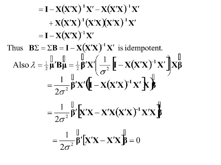
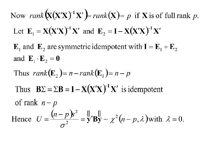
Comments The matrices are symmetric idempotent matrices also

Comments (continued)

Geometry of Least Squares

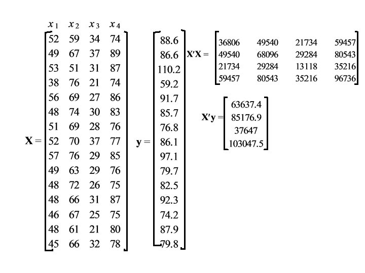
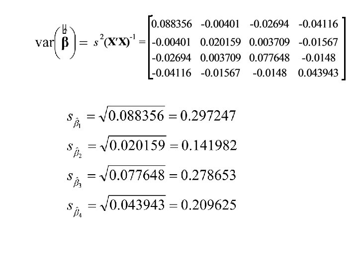
Example • Data is collected for n = 15 cases on the variables Y (the dependent variable) and X 1, X 2, X 3 and X 4. • The data and calculations are displayed on the next page:

Properties of The Maximum Likelihood Estimates Unbiasedness, Minimum Variance

Note: and Thus is an unbiased estimator of. Since is also a function of the set of complete minimal sufficient statistics, it is the UMVU estimator of. (Lehman-Scheffe)

Note: where In general

Thus: where

Thus:

Let Then Thus s 2 is an unbiased estimator of s 2. Since s 2 is also a function of the set of complete minimal sufficient statistics, it is the UMVU estimator of s 2.

Distributional Properties Least square Estimates (Maximum Likelidood estimates)

Recall 1. If ~ then A is a q × p matrix where

The General Linear Model The Estimates and

Theorem Proof

Finally and

Thus are independent. Summary

Example • Data is collected for n = 15 cases on the variables Y (the dependent variable) and X 1, X 2, X 3 and X 4. • The data and calculations are displayed on the next page:

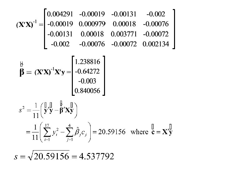
Estimates of the coefficients Compare with SPSS output

The General Linear Model with an intercept

Consider the random variable Y with 1. E[Y] = b 0+ b 1 X 1+ b 2 X 2 +. . . + bp. Xp (intercept included) and 2. var(Y) = s 2 • where b 1, b 2 , . . . , bp are unknown parameters • and X 1 , X 2 , . . . , Xp are nonrandom variables. • Assume further that Y is normally distributed.

The matrix formulation (intercept included) Then the model becomes Thus to include an intercept add an extra column of 1’s in the design matrix X and include the intercept in the parameter vector

The matrix formulation of the Simple Linear regression model

and Now

thus

Finally Thus

The Gauss-Markov Theorem An important result in theory of Linear models Proves optimality of Least squares estimates in a more general setting

Assume the following model Linear Model We will not necessarily assume Normality. Consider the least squares estimate of is an unbiased linear estimator of

The Gauss-Markov Theorem Assume Consider the least squares estimate of and , an unbiased linear estimator of Let denote any other unbiased linear estimator of

Proof Now

Now Also Thus is an unbiased estimator of if

Thus The Gauss-Markov theorem states that is the Best Linear Unbiased Estimator (B. L. U. E. ) of

Hypothesis testing for the GLM The General Linear Hypothesis

Testing the General Linear Hypotheses The General Linear Hypothesis h 11 b 1 + h 12 b 2 + h 13 b 3 +. . . + h 1 pbp = h 1 h 21 b 1 + h 22 b 2 + h 23 b 3 +. . . + h 2 pbp = h 2. . . hq 1 b 1 + hq 2 b 2 + hq 3 b 3 +. . . + hqpbp = hq where h 11, h 12, h 13, . . . , hqp and h 1, h 2, h 3, . . . , hq are known coefficients. In matrix notation H 0:

Examples 1. H 0: b 1 = 0 2. H 0: b 1 = 0, b 2 = 0, b 3 = 0 3. H 0: b 1 = b 2

Examples 4. H 0: b 1 = b 2 , b 3 = b 4 5. H 0: b 1 = 1/2(b 2 + b 3) 6. H 0: b 1 = 1/2(b 2 + b 3), b 3 = 1/3(b 4 + b 5 + b 6)

The. Likelihood Ratio Test The joint density of is: The likelihood function The log-likelihood function

Defn (Likelihood Ratio Test of size a) Rejects H 0: q w against the alternative hypothesis H 1: q w. when and K is chosen so that

Note We will maximize. The Lagrange multiplier technique will be used for this purpose

We will maximize.

or finally or

Thus the equations for are Now or and