ICS 415 Computer Graphics Hermite Splines Dr Muhammed

ICS 415 Computer Graphics Hermite Splines Dr. Muhammed Al-Mulhem March 1, 2009 Dr. Muhammed Al-Mulhem 1

Spline • A spline is a a flexible strip used to produce a smooth curve through a set of points. March 1, 2009 Dr. Muhammed Al-Mulhem 2

Representations of Curves • A curve can be represented using: – A sequence of points. – A piecewise polynomial functions. • A spline curve refers to any composite curve formed with polynomial sections. March 1, 2009 Dr. Muhammed Al-Mulhem 3

Specifying Curves • A spline curve is specified as follows: – Giving a set of coordinate positions, called control Points, which indicate the general shape of the curve. – These points are then fitted with piecewise polynomial functions in one of two ways: § Interpolation § Approximation March 1, 2009 Dr. Muhammed Al-Mulhem 4

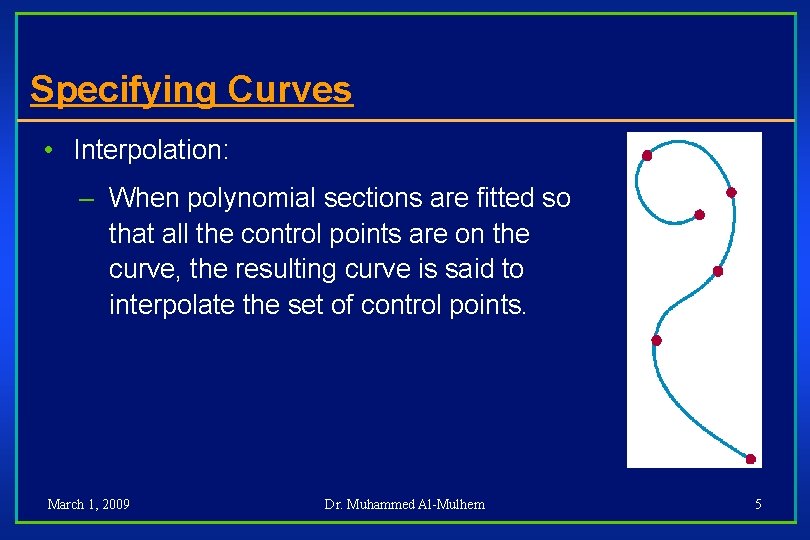
Specifying Curves • Interpolation: – When polynomial sections are fitted so that all the control points are on the curve, the resulting curve is said to interpolate the set of control points. March 1, 2009 Dr. Muhammed Al-Mulhem 5

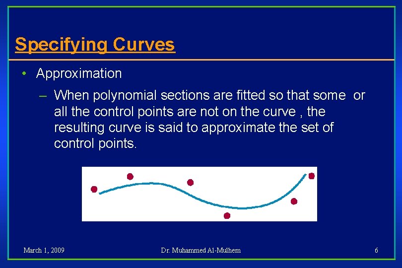
Specifying Curves • Approximation – When polynomial sections are fitted so that some or all the control points are not on the curve , the resulting curve is said to approximate the set of control points. March 1, 2009 Dr. Muhammed Al-Mulhem 6

Parametric Continuity • To ensure a smooth transition from one section of a piecewise parametric spline to the next, we impose various continuity conditions at the connection points. • If each section of a spline curve is described with a set of parametric coordinate function of the form x = x(u), y= y(u), z = z(u), • u 1 <= u 2 We set parametric continuity by matching the parametric derivatives of adjoining curve sections at their common boundary. March 1, 2009 Dr. Muhammed Al-Mulhem 7

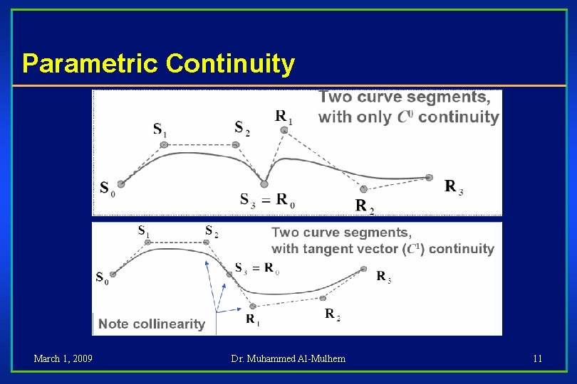
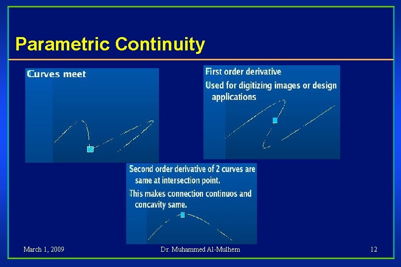
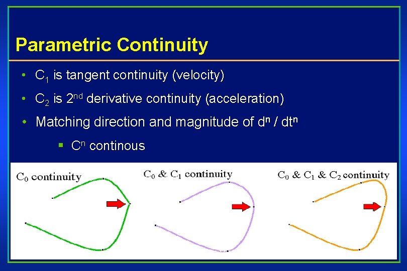
Parametric Continuity • Various continuity conditions: • C 0 continuity (Zero-order parametric continuity): – Means simply that curves meet. That is, the values of x, y, and z evaluated at u 2 for the first curve section are equal, respectively, to the values of x, y, and z evaluated at u 1 of the next curve section. March 1, 2009 Dr. Muhammed Al-Mulhem 8

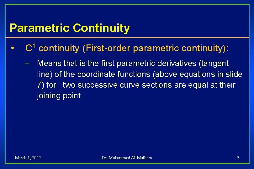
Parametric Continuity • C 1 continuity (First-order parametric continuity): – Means that is the first parametric derivatives (tangent line) of the coordinate functions (above equations in slide 7) for two successive curve sections are equal at their joining point. March 1, 2009 Dr. Muhammed Al-Mulhem 9

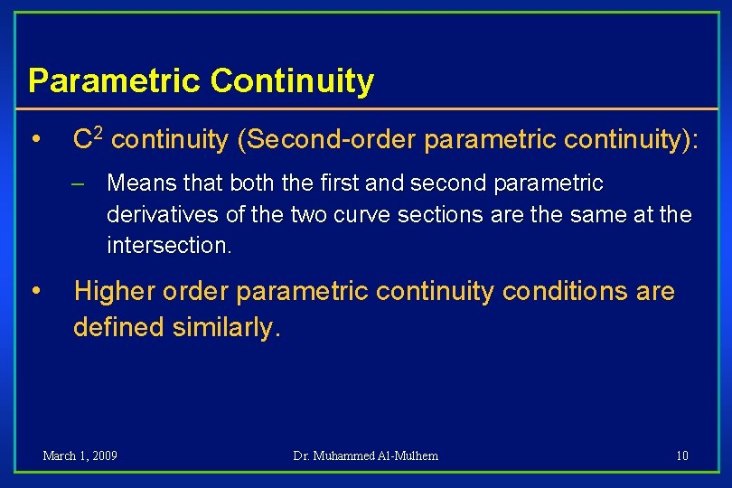
Parametric Continuity • C 2 continuity (Second-order parametric continuity): – Means that both the first and second parametric derivatives of the two curve sections are the same at the intersection. • Higher order parametric continuity conditions are defined similarly. March 1, 2009 Dr. Muhammed Al-Mulhem 10

Parametric Continuity March 1, 2009 Dr. Muhammed Al-Mulhem 11

Parametric Continuity March 1, 2009 Dr. Muhammed Al-Mulhem 12

Cubic Spline • Cubic spline requires less calculations and storage space, and more stable than higher-order polynomials. • Given a set of control points, cubic interpolation splines are obtained by fitting the input points with a piecewise cubic polynomial curve that passes through every control point. March 1, 2009 Dr. Muhammed Al-Mulhem 13

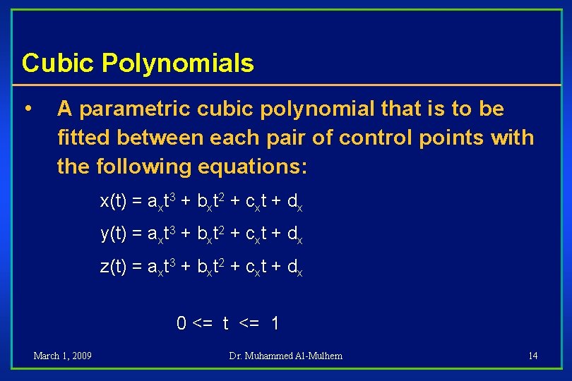
Cubic Polynomials • A parametric cubic polynomial that is to be fitted between each pair of control points with the following equations: x(t) = axt 3 + bxt 2 + cxt + dx y(t) = axt 3 + bxt 2 + cxt + dx z(t) = axt 3 + bxt 2 + cxt + dx 0 <= t <= 1 March 1, 2009 Dr. Muhammed Al-Mulhem 14

Cubic Polynomials Let T = [t 3 t 2 t 1] Coefficient Matrix C The the cuve Q(t) can be represented as: Q(t) = T*C March 1, 2009 Dr. Muhammed Al-Mulhem 15

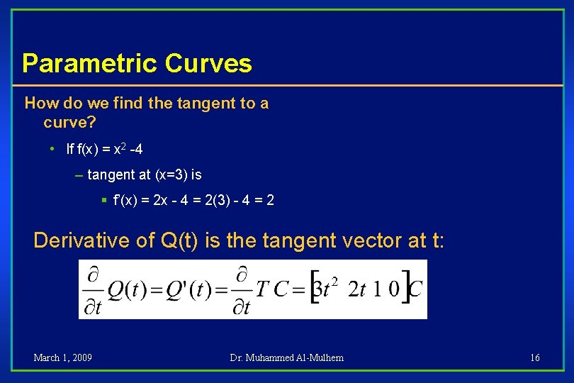
Parametric Curves How do we find the tangent to a curve? • If f(x) = x 2 -4 – tangent at (x=3) is § f’(x) = 2 x - 4 = 2(3) - 4 = 2 Derivative of Q(t) is the tangent vector at t: March 1, 2009 Dr. Muhammed Al-Mulhem 16

Piecewise Curve Segments One curve constructed by connecting many smaller segments end-to-end • Must have rules for how the segments are joined Continuity describes the joint • Parametric continuity • Geometric continuity March 1, 2009 Dr. Muhammed Al-Mulhem 17

Parametric Continuity • C 1 is tangent continuity (velocity) • C 2 is 2 nd derivative continuity (acceleration) • Matching direction and magnitude of dn / dtn § Cn continous March 1, 2009 Dr. Muhammed Al-Mulhem 18

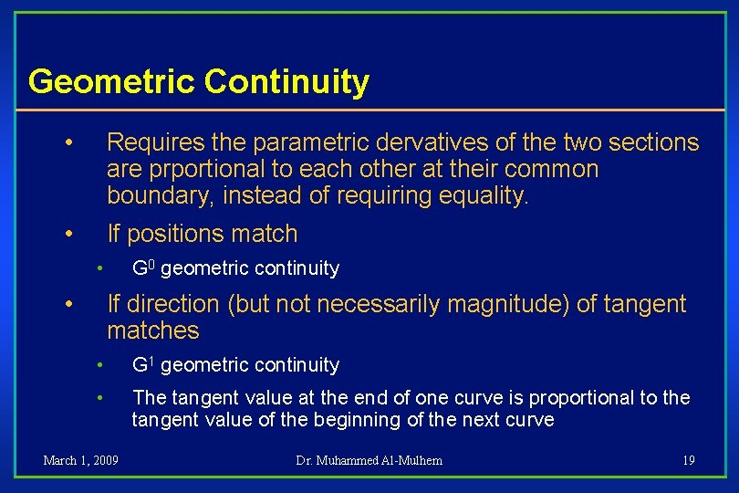
Geometric Continuity • Requires the parametric dervatives of the two sections are prportional to each other at their common boundary, instead of requiring equality. • If positions match • • G 0 geometric continuity If direction (but not necessarily magnitude) of tangent matches • G 1 geometric continuity • The tangent value at the end of one curve is proportional to the tangent value of the beginning of the next curve March 1, 2009 Dr. Muhammed Al-Mulhem 19

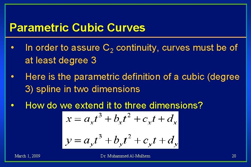
Parametric Cubic Curves • In order to assure C 2 continuity, curves must be of at least degree 3 • Here is the parametric definition of a cubic (degree 3) spline in two dimensions • How do we extend it to three dimensions? March 1, 2009 Dr. Muhammed Al-Mulhem 20

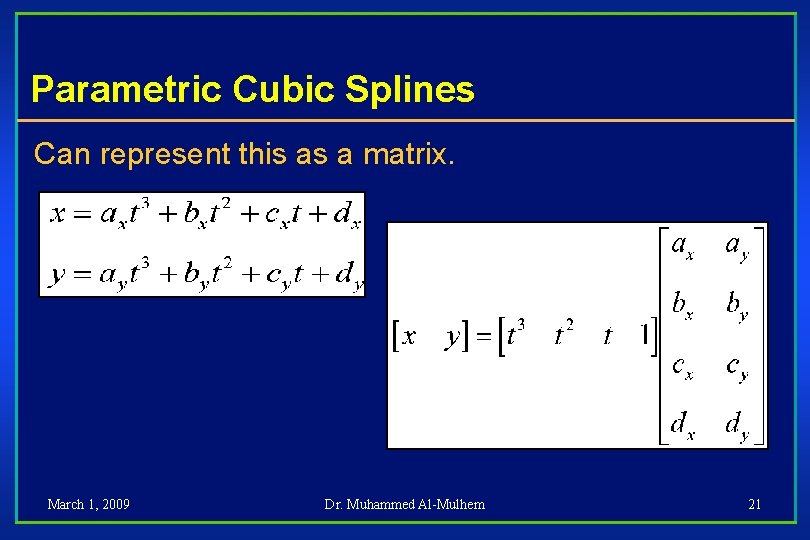
Parametric Cubic Splines Can represent this as a matrix. March 1, 2009 Dr. Muhammed Al-Mulhem 21

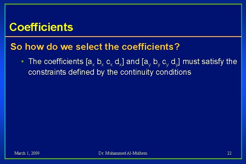
Coefficients So how do we select the coefficients? • The coefficients [ax bx cx dx] and [ay by cy dy] must satisfy the constraints defined by the continuity conditions March 1, 2009 Dr. Muhammed Al-Mulhem 22

Parametric Curves • There are many splines developed, some of these are: – Hermite – Bezier March 1, 2009 Dr. Muhammed Al-Mulhem 23

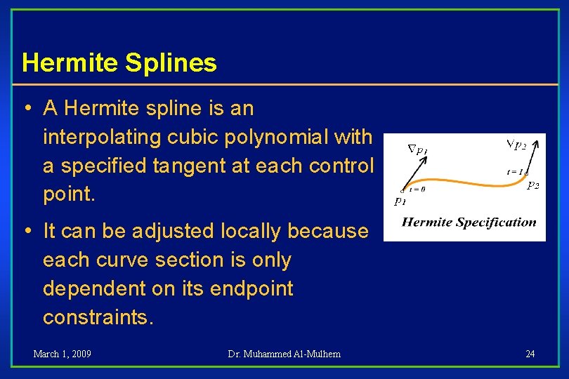
Hermite Splines • A Hermite spline is an interpolating cubic polynomial with a specified tangent at each control point. • It can be adjusted locally because each curve section is only dependent on its endpoint constraints. March 1, 2009 Dr. Muhammed Al-Mulhem 24

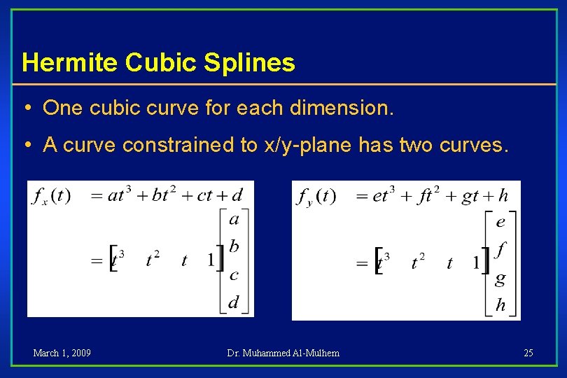
Hermite Cubic Splines • One cubic curve for each dimension. • A curve constrained to x/y-plane has two curves. March 1, 2009 Dr. Muhammed Al-Mulhem 25

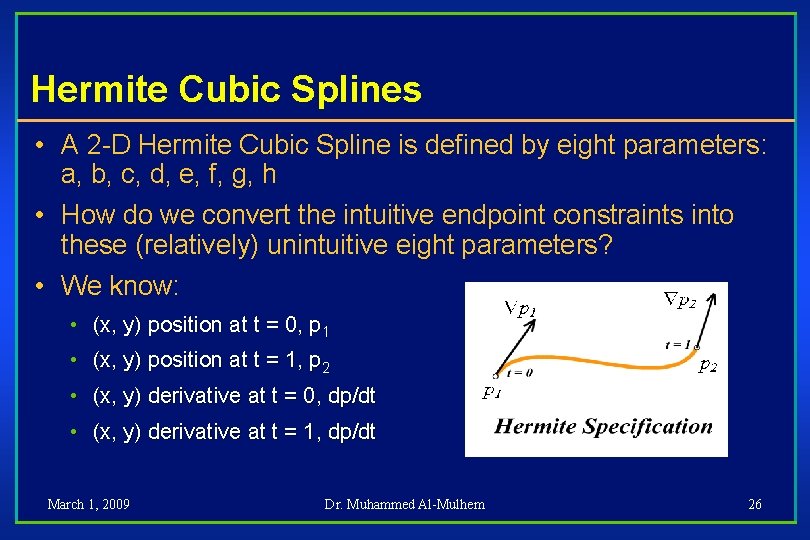
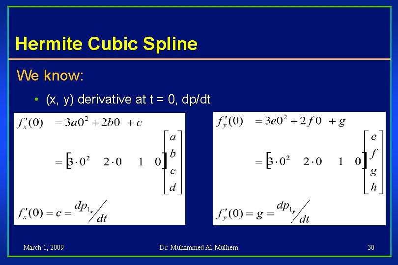
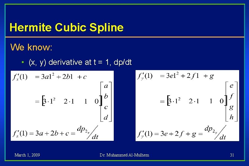
Hermite Cubic Splines • A 2 -D Hermite Cubic Spline is defined by eight parameters: a, b, c, d, e, f, g, h • How do we convert the intuitive endpoint constraints into these (relatively) unintuitive eight parameters? • We know: • (x, y) position at t = 0, p 1 • (x, y) position at t = 1, p 2 • (x, y) derivative at t = 0, dp/dt • (x, y) derivative at t = 1, dp/dt March 1, 2009 Dr. Muhammed Al-Mulhem 26

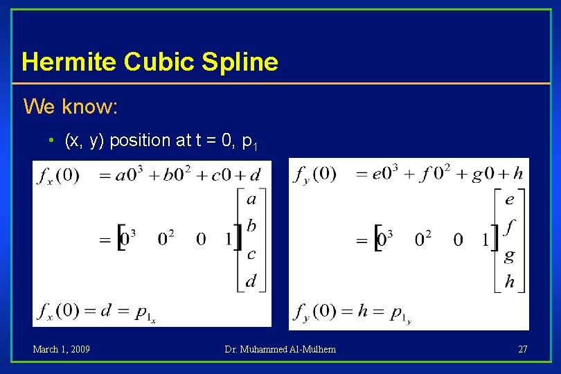
Hermite Cubic Spline We know: • (x, y) position at t = 0, p 1 March 1, 2009 Dr. Muhammed Al-Mulhem 27

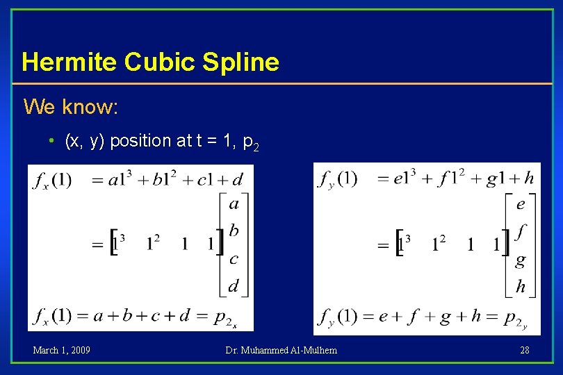
Hermite Cubic Spline We know: • (x, y) position at t = 1, p 2 March 1, 2009 Dr. Muhammed Al-Mulhem 28

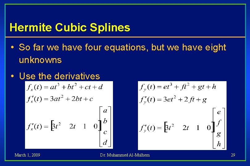
Hermite Cubic Splines • So far we have four equations, but we have eight unknowns • Use the derivatives March 1, 2009 Dr. Muhammed Al-Mulhem 29

Hermite Cubic Spline We know: • (x, y) derivative at t = 0, dp/dt March 1, 2009 Dr. Muhammed Al-Mulhem 30

Hermite Cubic Spline We know: • (x, y) derivative at t = 1, dp/dt March 1, 2009 Dr. Muhammed Al-Mulhem 31

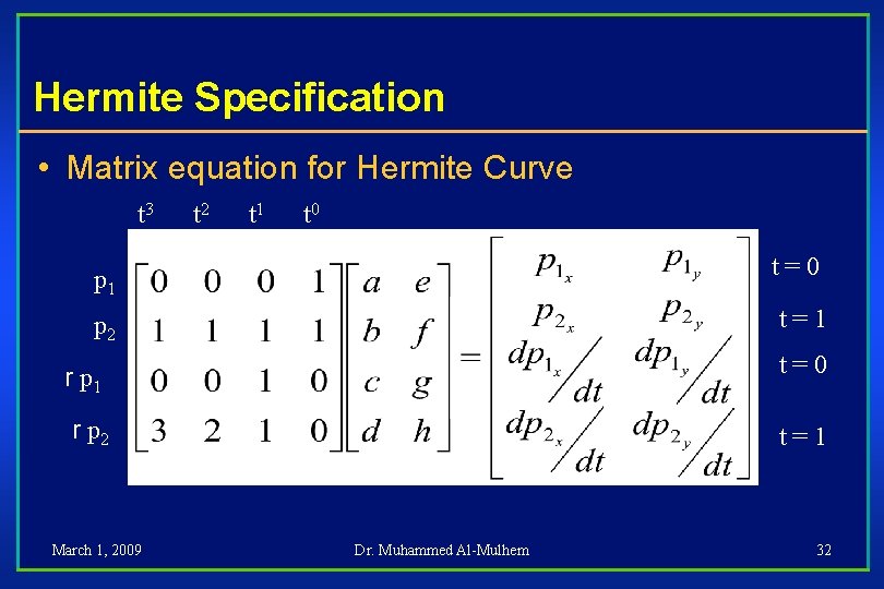
Hermite Specification • Matrix equation for Hermite Curve t 3 t 2 t 1 t 0 p 1 t=0 p 2 t=1 r p 1 t=0 r p 2 t=1 March 1, 2009 Dr. Muhammed Al-Mulhem 32

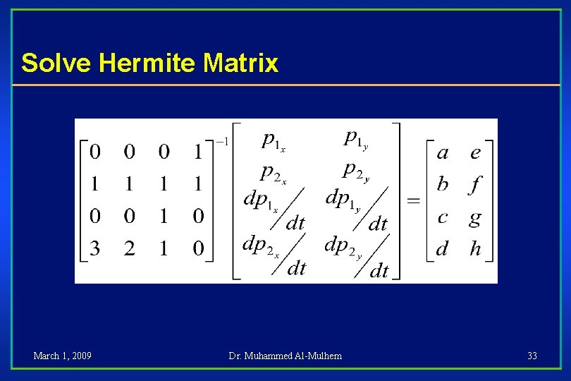
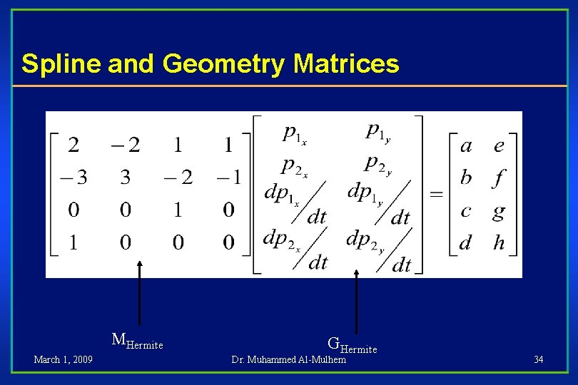
Solve Hermite Matrix March 1, 2009 Dr. Muhammed Al-Mulhem 33

Spline and Geometry Matrices MHermite March 1, 2009 GHermite Dr. Muhammed Al-Mulhem 34

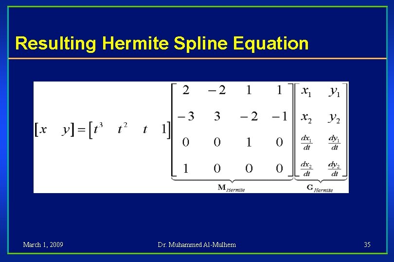
Resulting Hermite Spline Equation March 1, 2009 Dr. Muhammed Al-Mulhem 35

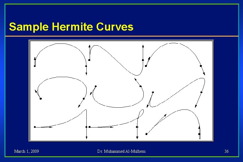
Sample Hermite Curves March 1, 2009 Dr. Muhammed Al-Mulhem 36

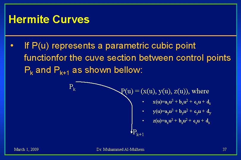
Hermite Curves • If P(u) represents a parametric cubic point functionfor the cuve section between control points Pk and Pk+1 as shown bellow: Pk P(u) = (x(u), y(u), z(u)), where • x(u)=axu 3 + bxu 2 + cxu + dx • y(u)=ayu 3 + byu 2 + cyu + dy • z(u)=azu 3 + bzu 2 + czu + dz Pk+1 March 1, 2009 Dr. Muhammed Al-Mulhem 37

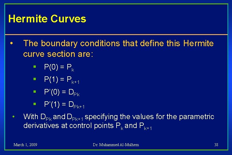
Hermite Curves • The boundary conditions that define this Hermite curve section are: § P(0) = Pk § P(1) = Pk+1 § P’(0) = DPk § P’(1) = DPk+1 • With DPk and DPk+1 specifying the values for the parametric derivatives at control points Pk and Pk+1 March 1, 2009 Dr. Muhammed Al-Mulhem 38

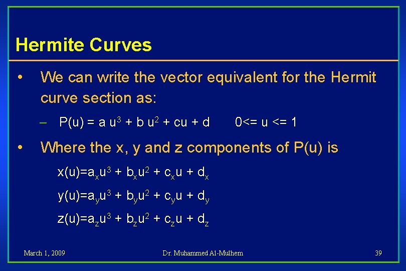
Hermite Curves • We can write the vector equivalent for the Hermit curve section as: – P(u) = a u 3 + b u 2 + cu + d • 0<= u <= 1 Where the x, y and z components of P(u) is x(u)=axu 3 + bxu 2 + cxu + dx y(u)=ayu 3 + byu 2 + cyu + dy z(u)=azu 3 + bzu 2 + czu + dz March 1, 2009 Dr. Muhammed Al-Mulhem 39

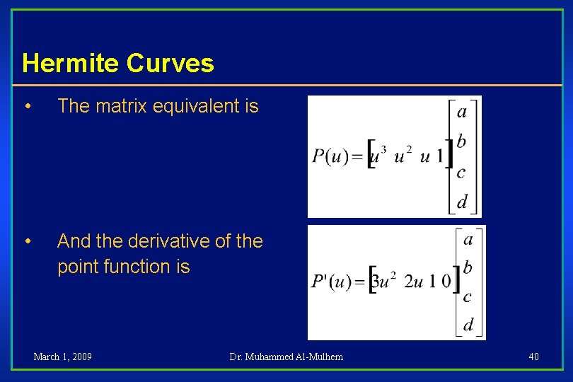
Hermite Curves • The matrix equivalent is • And the derivative of the point function is March 1, 2009 Dr. Muhammed Al-Mulhem 40

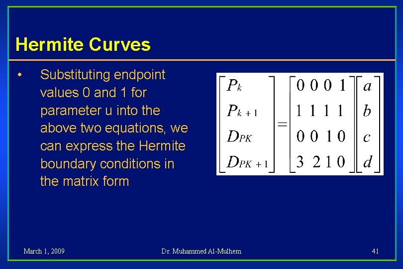
Hermite Curves • Substituting endpoint values 0 and 1 for parameter u into the above two equations, we can express the Hermite boundary conditions in the matrix form March 1, 2009 Dr. Muhammed Al-Mulhem 41

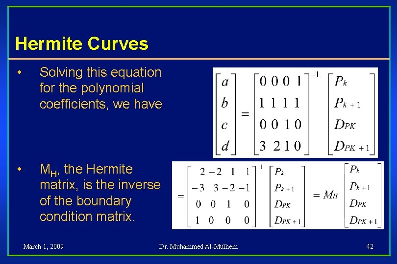
Hermite Curves • Solving this equation for the polynomial coefficients, we have • MH, the Hermite matrix, is the inverse of the boundary condition matrix. March 1, 2009 Dr. Muhammed Al-Mulhem 42

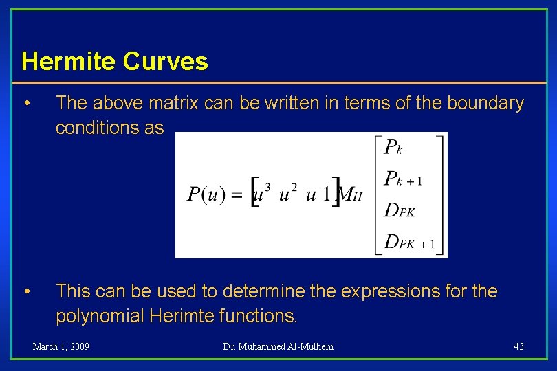
Hermite Curves • The above matrix can be written in terms of the boundary conditions as • This can be used to determine the expressions for the polynomial Herimte functions. March 1, 2009 Dr. Muhammed Al-Mulhem 43

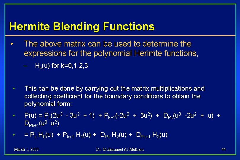
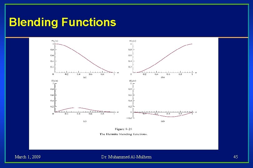
Hermite Blending Functions • The above matrix can be used to determine the expressions for the polynomial Herimte functions, – Hk(u) for k=0, 1, 2, 3 • This can be done by carrying out the matrix multiplications and collecting coefficient for the boundary conditions to obtain the polynomial form: • P(u) = Pk(2 u 3 - 3 u 2 + 1) + Pk+1(-2 u 3 + 3 u 2) + DPk(u 3 -2 u 2 + u) + DPk+1(u 3 u 2) • = Pk H 0(u) + Pk+1 H 1(u) + DPk H 2(u) + DPk+1 H 3(u) March 1, 2009 Dr. Muhammed Al-Mulhem 44

Blending Functions March 1, 2009 Dr. Muhammed Al-Mulhem 45