MayaDemo 2020116 12 Hermite Hermite Curve Interpolation Hermite


 Hermite curve • • • Continuity between beginning and ending tangent")


![CSpline Code CSpline: : CSpline(int x[100], int y[100], int n, int grain, float tension)](https://slidetodoc.com/presentation_image/5d352bd4293e6d37e7447a9642191dbd/image-46.jpg "CSpline Code CSpline: : CSpline(int x[100], int y[100], int n, int grain, float tension)")
 { CPt")
![void CSpline: : Get. Cardinal. Matrix(float a 1) { m[0]=-a 1; m[1]=2. -a 1;](https://slidetodoc.com/presentation_image/5d352bd4293e6d37e7447a9642191dbd/image-48.jpg "void CSpline: : Get. Cardinal. Matrix(float a 1) { m[0]=-a 1; m[1]=2. -a 1;")


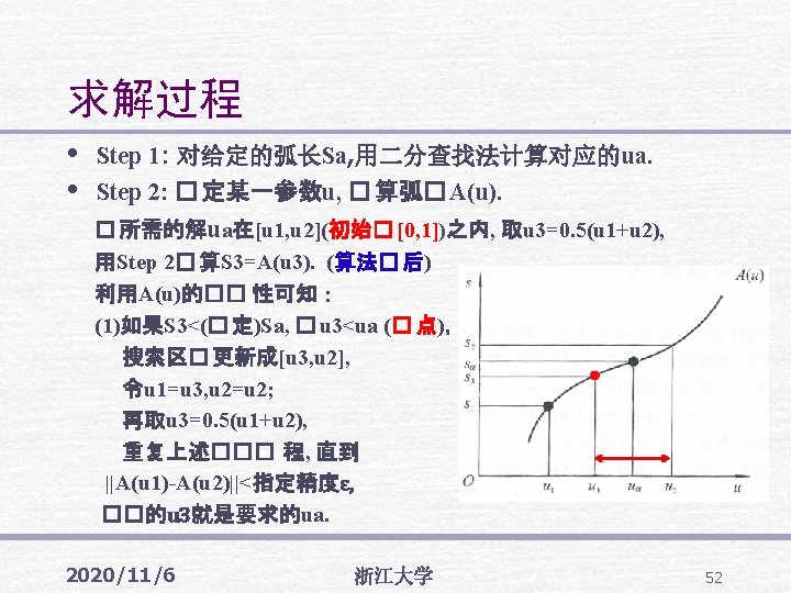
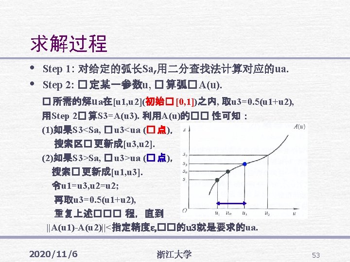

, (0, y 1), (h, y 2)")
 is continuous")


- Slides: 68
Maya动画Demo 2020/11/6 浙江大学 12
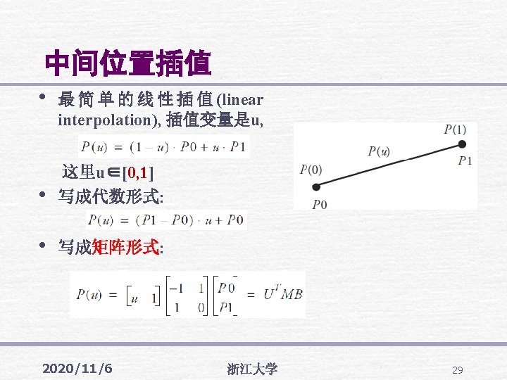
插值函数—选择Hermite曲线 • Hermite Curve Interpolation • Hermite interpolation generates a cubic • polynomial from one point to another. They are used to smoothly interpolate between key -points (like object movement in keyframe animation or camera control). Understanding the mathematical background of Hermite curves will help you to understand the entire family of splines. 2020/11/6 浙江大学 34
The Math • We only talk about 2 -D curves here. To calculate a hermite curve we need the following vectors: • Pi: the startpoint of the curve • P’i: the tangent (e. g. direction and speed) to • • how the curve leaves the startpoint Pi+1: the endpoint of the curve P’i+1: the tangent (e. g. direction and speed) to how the curves meets the endpoint 2020/11/6 浙江大学 35
Hermite basis • These 4 vectors are simply multiplied with 4 Hermite basis functions and added together. h 1(u) = 2 u^3 – 3 u^2 + 1 h 2(u) = -2 u^3 + 3 u^2 h 3(u) = u^3 – 2 u^2 + u h 4(u) = u^3 - u^2 Below are the 4 graphs of the 4 functions (from left to right: h 1, h 2, h 3, h 4). (把u=0, 0. 5和1代入上面公式中估计图 形上的位置) (all graphs except the 4 th have been plotted from 0, 0 to 1, 1) 2020/11/6 浙江大学 36
The Math in Matrix Form • • All this stuff can be expressed with some vector and matrix algebra. Vector U: The interpolation-point and it's powers up to 3; Matrix M: The matrix form of the 4 hermite polynomials; Vector B: The parameters of our hermite curve; 它们确定 了从起始点到终止点两点之间的曲线形状 2020/11/6 浙江大学 37
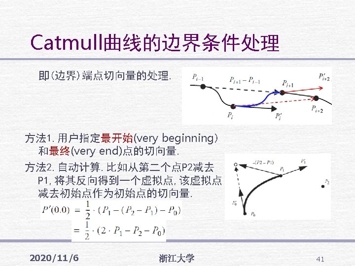
A composite (合成) Hermite curve • • • Continuity between beginning and ending tangent vectors of connected segments is ensured by merely using the ending tangent vector of one segment as the beginning tangent vector of the next. A composite Hermite curve (piecewise cubic with first-order continuity at the junctions) is shown bellow. However, specifying all of the needed tangent vectors can be a burden! 2020/11/6 浙江大学 38
Catmull-Rom Spline • The Catmull-Rom curve can be viewed as a Hermite curve in which the tangents at the interior control points are automatically generated according to a relatively simple geometric procedure. 2020/11/6 浙江大学 39
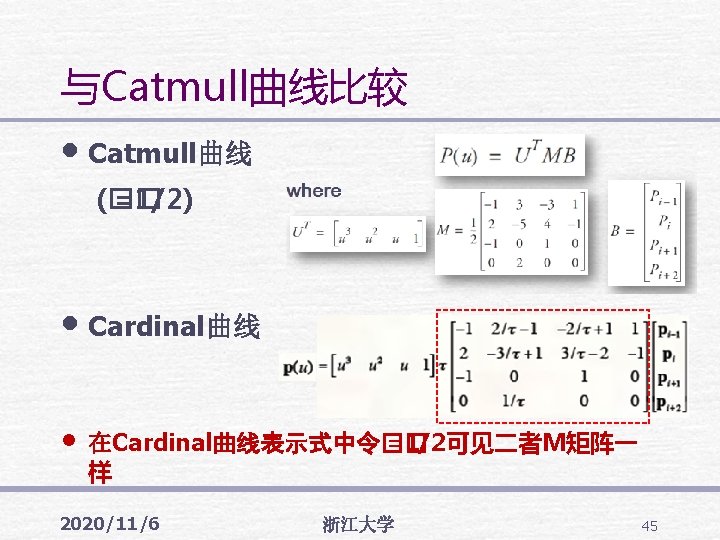
Matrix form of Catmull-Rom Spline where • Catmull-Rom spline is a special type of Cardinal spline(下面要讲), 注意M, B均变化了. 2020/11/6 浙江大学 40
Cardinal Spline • • Cardinal Splines are just a subset of the Hermite curves. They don‘t need the tangent points because they will be calculated from the control points. The formula for the tangents for cardinal splines is: P’i = τ* ( Pi+1 - Pi-1 ) τ is a constant which affects the tightness of the curve. and τ =0. 5 in Catmull spline. 2020/11/6 浙江大学 43
From Hermite to Cardinal spline 2020/11/6 浙江大学 44
CSpline Code CSpline: : CSpline(int x[100], int y[100], int n, int grain, float tension) //x[], y[]控制点坐标, n 为控制点数量, grain为控制点之间的插值平滑点, tension为通过控制点位值的曲线平滑程度. { int i, np; n 0=n+1; np=n 0; CPt jd[100]; CPt *knots; knots 0=knots; for(i=1; i<=np; i++) { jd[i]. x = x[i-1]; jd[i]. y = y[i-1]; } jd[0]. x = x[0]; jd[0]. y = y[0]; jd[np+1]. x = x[np-1]; jd[np+1]. y = y[np-1]; np=np+2; knots=jd; (自己考察首尾两个点上不重复赋值会有什么结果) Cubic. Spline(np, knots, grain, tension); } 2020/11/6 浙江大学 46
void CSpline: : Cubic. Spline(int n, CPt *knots, int grain, float tension) { CPt *s, *k 0, *kml, *k 1, *k 2; int i, j; float alpha[30]; Get. Cardinal. Matrix(tension); for(i=0; i<grain; i++) u[i] =((float)i)/grain; //u∈[0, 1] s = Spline; kml = knots; k 0=kml+1; k 1=k 0+1; k 2=k 1+1; for(i=1; i<n-1; i++) { for(j=0; j<grain; j++) { s->x = Matrix(kml->x, k 0 ->x, k 1 ->x, k 2 ->x, u[j] ); s->y = Matrix(kml->y, k 0 ->y, k 1 ->y, k 2 ->y, u[j] ); s->z = Matrix(kml->z, k 0 ->z, k 1 ->z, k 2 ->z, u[j] ); s++; } k 0++; kml++; k 1++; k 2++; } } 注: 如果输入的控制点就是 3 D的, 该程序也能生成 3 D样条曲线, 作业: 对照程序代码和矩阵表示的关系. 2020/11/6 浙江大学 47
void CSpline: : Get. Cardinal. Matrix(float a 1) { m[0]=-a 1; m[1]=2. -a 1; m[2]=a 1 -2. ; m[3]=a 1; m[4]=2. *a 1; m[5]=a 1 -3. ; m[6]=3. -2*a 1; m[7]=-a 1; m[8]=-a 1; m[9]=0. ; m[10]=a 1; m[11]=0. ; m[12]=0. ; m[13]=1. ; m[14]=0. ; m[15]=0. ; } float CSpline: : Matrix(float a, float b, float c, float d, float u) { float p 0, p 1, p 2, p 3; p 0=m[0]*a+m[1]*b+m[2]*c+m[3]*d; p 1=m[4]*a+m[5]*b+m[6]*c+m[7]*d; p 2=m[8]*a+m[9]*b+m[10]*c+m[11]*d; p 3=m[12]*a+m[13]*b+m[14]*c+m[15]*d; return(p 3+u*(p 2+u*(p 1+u*p 0))); } 浙江大学 48
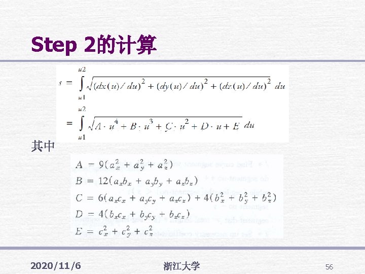
用扩展的Simpson方法计算积分 • • Simpson Rule is a numerical method that approximates the value of a definite integral by using quadratic (二次的) polynomials. Let’s first derive a formula for the area under a parabola of equation y = ax^2 + bx + c passing through the three points: (−h, y 0), (0, y 1), (h, y 2). 2020/11/6 浙江大学 58
用扩展的Simpson方法计算积分 • Since the points (−h, y 0), (0, y 1), (h, y 2) are on the parabola, they satisfy y = ax^2 + bx + c. Therefore, • Observe that • Therefore, the area under the parabola is 2020/11/6 浙江大学 59
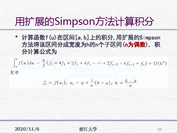
用扩展的Simpson方法计算积分 • We consider the definite integral • We assume that f(x) is continuous on [a, b] and we divide [a, b] into an even number n of subintervals of equal length • using the n + 1 points • We can compute the value of f(x) at these points. 2020/11/6 浙江大学 60
用扩展的Simpson方法计算积分 • We can estimate the integral by adding the areas under the parabolic arcs through three successive points. • By simplifying, we obtain Simpson’s rule formula. 2020/11/6 浙江大学 61