Hypothesis tests III Statistical errors oneand two sided

Hypothesis tests III. Statistical errors, one-and two sided tests. One-way analysis of variance.

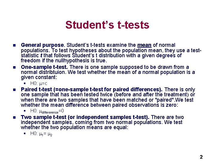
Student’s t-tests n n General purpose. Student’s t-tests examine the mean of normal populations. To test hypotheses about the population mean, they use a teststatistic t that follows Student’s t distribution with a given degrees of freedom if the nullhypothesis is true. One-sample t-test. There is one sample supposed to be drawn from a normal distribtuion. We test whether the mean of a normal population is a given constant: § H 0: =c n Paired t-test (=one-sample t-test for paired differences). There is only one sample that has been tested twice (before and after the treatment) or when there are two samples that have been matched or "paired". We test whether the mean difference between paired observations is zero: § H 0: differerence=0 n Two sample t-test (or independent samples t-test). There are two independent samples, coming from two normal populations. We test whether the two population means are equal: § H 0: 1= 2 2

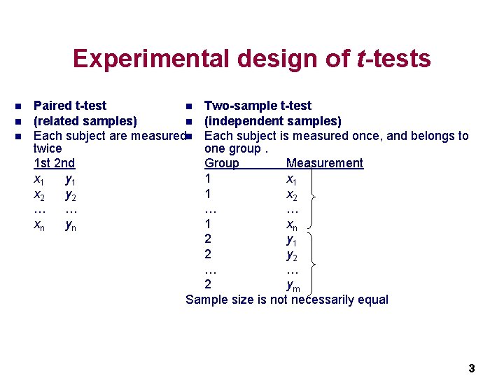
Experimental design of t-tests n n n Paired t-test n (related samples) n Each subject are measuredn twice 1 st 2 nd x 1 y 1 x 2 y 2 … … xn yn Two-sample t-test (independent samples) Each subject is measured once, and belongs to one group. Group Measurement 1 x 1 1 x 2 … … 1 xn 2 y 1 2 y 2 … … 2 ym Sample size is not necessarily equal 3

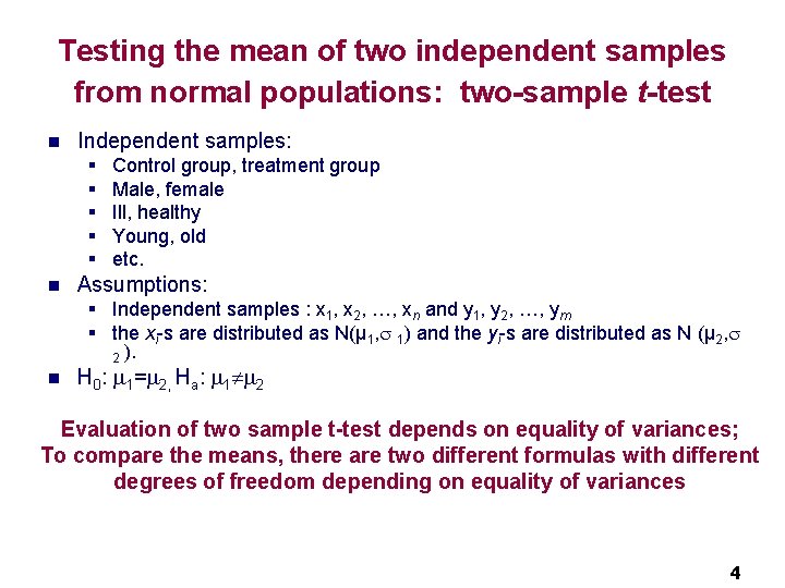
Testing the mean of two independent samples from normal populations: two-sample t-test n Independent samples: § § § n Control group, treatment group Male, female Ill, healthy Young, old etc. Assumptions: § Independent samples : x 1, x 2, …, xn and y 1, y 2, …, ym § the xi-s are distributed as N(µ 1, 1) and the yi-s are distributed as N (µ 2, 2 ). n H 0: 1= 2, Ha: 1 2 Evaluation of two sample t-test depends on equality of variances; To compare the means, there are two different formulas with different degrees of freedom depending on equality of variances 4

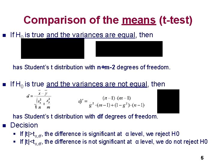
Comparison of the means (t-test) n If H 0 is true and the variances are equal, then has Student’s t distribution with n+m-2 degrees of freedom. n If H 0 is true and the variances are not equal, then. has Student’s t distribution with df degrees of freedom. n Decision § If |t|>tα, df, the difference is significant at α level, we reject H 0 § If |t|<tα, df, the difference is not significant at α level, we do not reject H 0 5

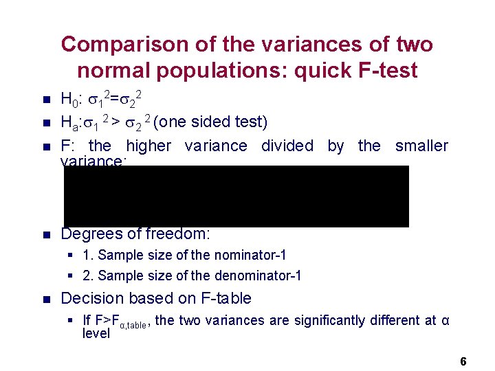
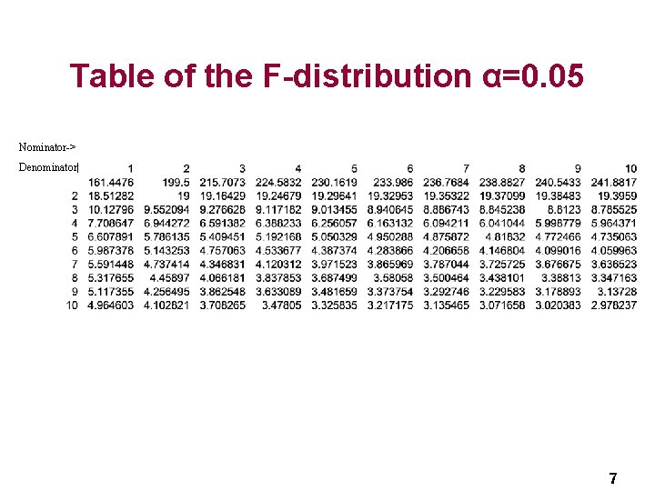
Comparison of the variances of two normal populations: quick F-test n n H 0: 12= 22 Ha: 1 2 > 2 2 (one sided test) F: the higher variance divided by the smaller variance: Degrees of freedom: § 1. Sample size of the nominator-1 § 2. Sample size of the denominator-1 n Decision based on F-table § If F>Fα, table, the two variances are significantly different at α level 6

Table of the F-distribution α=0. 05 Nominator-> Denominator| 7

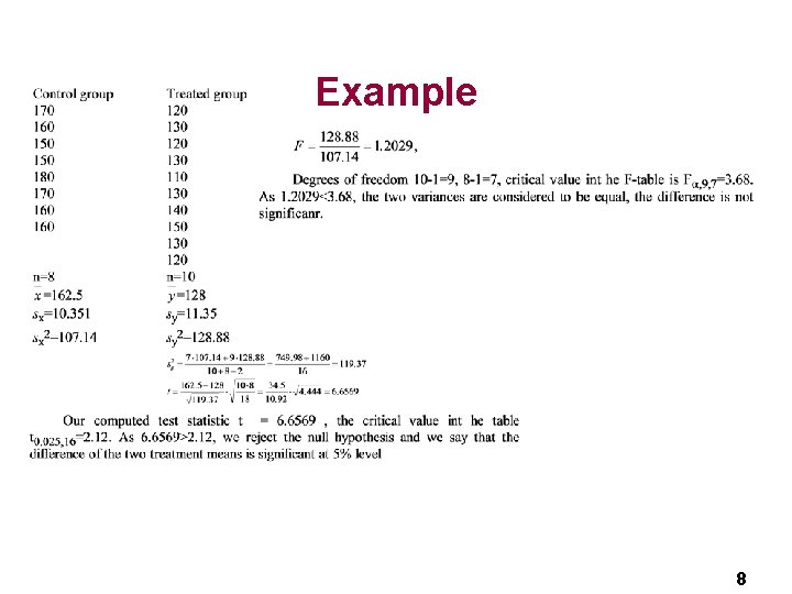
Example 8

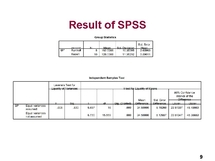
Result of SPSS 9

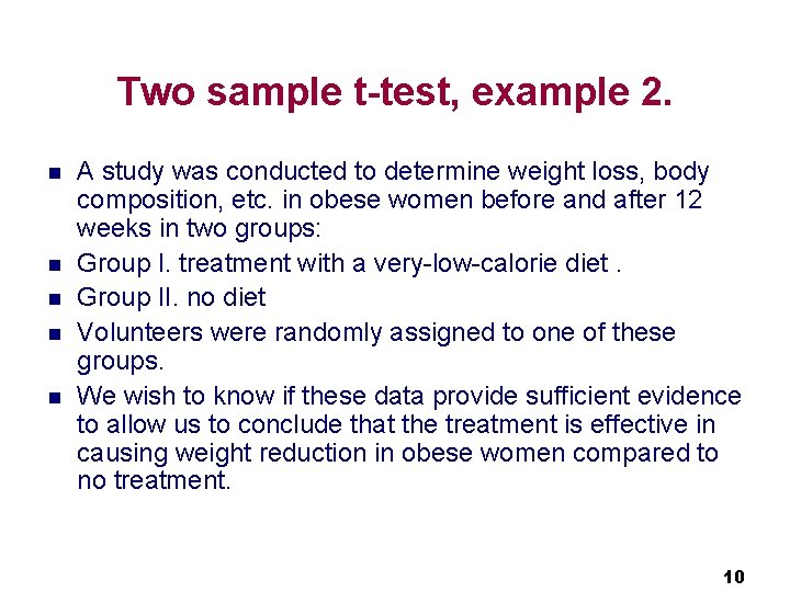
Two sample t-test, example 2. n n n A study was conducted to determine weight loss, body composition, etc. in obese women before and after 12 weeks in two groups: Group I. treatment with a very-low-calorie diet. Group II. no diet Volunteers were randomly assigned to one of these groups. We wish to know if these data provide sufficient evidence to allow us to conclude that the treatment is effective in causing weight reduction in obese women compared to no treatment. 10

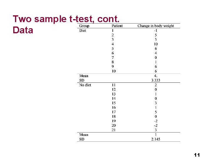
Two sample t-test, cont. Data 11

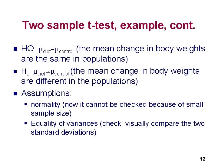
Two sample t-test, example, cont. n n n HO: diet= control, (the mean change in body weights are the same in populations) Ha: diet control (the mean change in body weights are different in the populations) Assumptions: § normality (now it cannot be checked because of small sample size) § Equality of variances (check: visually compare the two standard deviations) 12

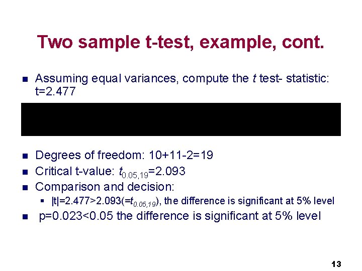
Two sample t-test, example, cont. n Assuming equal variances, compute the t test- statistic: t=2. 477 n Degrees of freedom: 10+11 -2=19 Critical t-value: t 0. 05, 19=2. 093 Comparison and decision: n n § |t|=2. 477>2. 093(=t 0. 05, 19), the difference is significant at 5% level n p=0. 023<0. 05 the difference is significant at 5% level 13

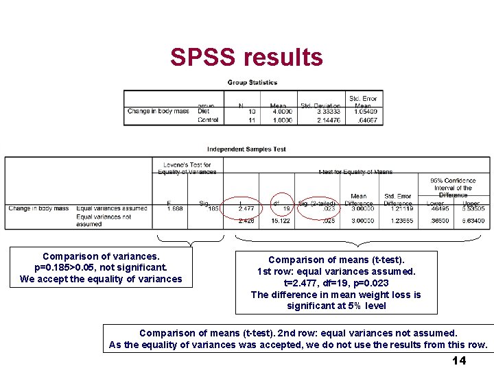
SPSS results Comparison of variances. p=0. 185>0. 05, not significant. We accept the equality of variances Comparison of means (t-test). 1 st row: equal variances assumed. t=2. 477, df=19, p=0. 023 The difference in mean weight loss is significant at 5% level Comparison of means (t-test). 2 nd row: equal variances not assumed. As the equality of variances was accepted, we do not use the results from this row. 14

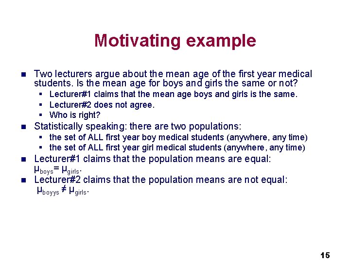
Motivating example n Two lecturers argue about the mean age of the first year medical students. Is the mean age for boys and girls the same or not? § Lecturer#1 claims that the mean age boys and girls is the same. § Lecturer#2 does not agree. § Who is right? n Statistically speaking: there are two populations: § the set of ALL first year boy medical students (anywhere, any time) § the set of ALL first year girl medical students (anywhere, any time) n n Lecturer#1 claims that the population means are equal: μboys= μgirls. Lecturer#2 claims that the population means are not equal: μboyys ≠ μgirls. 15

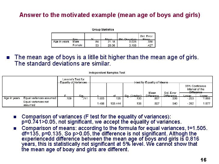
Answer to the motivated example (mean age of boys and girls) n The mean age of boys is a litlle bit higher than the mean age of girls. The standard deviations are similar. n n Comparison of variances (F test for the equality of variances): p=0. 741>0. 05, not significant, we accept the equality of variances. Comparison of means: according to the formula for equal variances, t=1. 505. df=135, p=0. 135. So p>0. 05, the difference is not significant. Althogh the experiencedd difference between the mean age of boys and girls is 0. 816 years, this is statistically not significant at 5% level. We cannot show that the mean age of boay and girls are different. 16

Other aspects of statistical tests 17

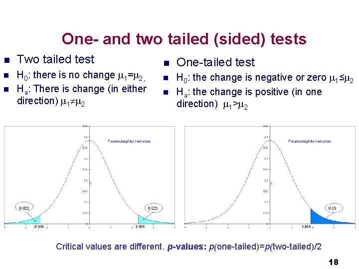
One- and two tailed (sided) tests n Two tailed test n H 0: there is no change 1= 2, Ha: There is change (in either direction) 1 2 n n One-tailed test n H 0: the change is negative or zero 1≤ 2 Ha: the change is positive (in one direction) 1> 2 n Critical values are different. p-values: p(one-tailed)=p(two-tailed)/2 18

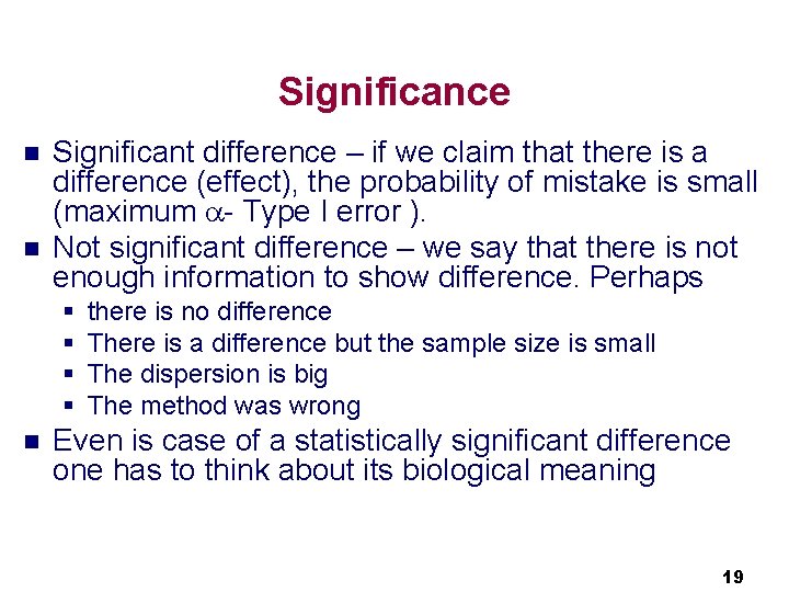
Significance n n Significant difference – if we claim that there is a difference (effect), the probability of mistake is small (maximum - Type I error ). Not significant difference – we say that there is not enough information to show difference. Perhaps § § n there is no difference There is a difference but the sample size is small The dispersion is big The method was wrong Even is case of a statistically significant difference one has to think about its biological meaning 19

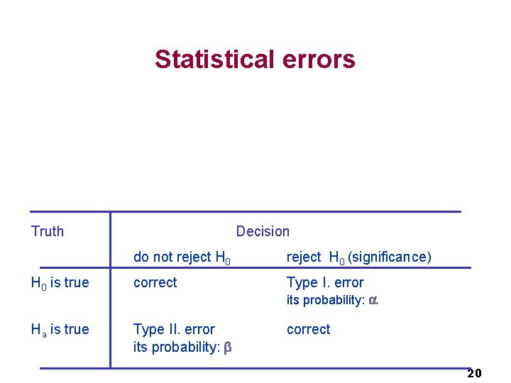
Statistical errors Truth Decision do not reject H 0 (significance) H 0 is true correct Type I. error Ha is true Type II. error its probability: correct its probability: 20

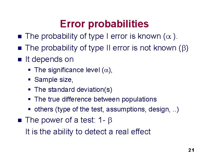
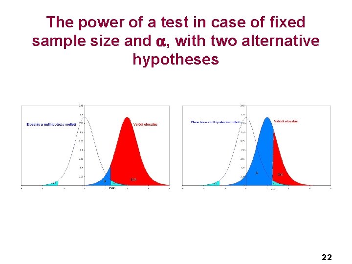
Error probabilities n n n The probability of type I error is known ( ). The probability of type II error is not known ( ) It depends on § § § n The significance level ( ), Sample size, The standard deviation(s) The true difference between populations others (type of the test, assumptions, design, . . ) The power of a test: 1 - It is the ability to detect a real effect 21

The power of a test in case of fixed sample size and , with two alternative hypotheses 22

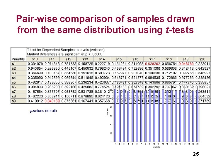
Comparison of several samples The repeated use of t-tests is not appropriate 23

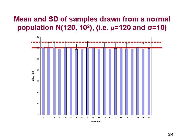
Mean and SD of samples drawn from a normal population N(120, 102), (i. e. =120 and σ=10) 24

Pair-wise comparison of samples drawn from the same distribution using t-tests p-values (detail) 25

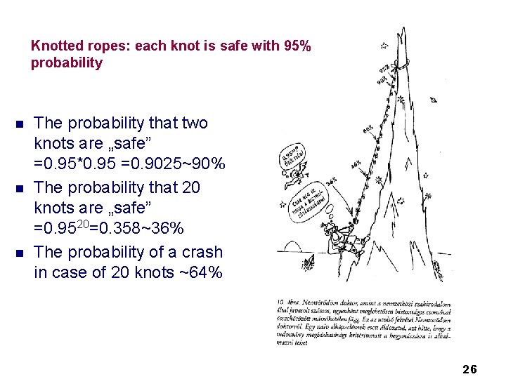
Knotted ropes: each knot is safe with 95% probability n n n The probability that two knots are „safe” =0. 95*0. 95 =0. 9025~90% The probability that 20 knots are „safe” =0. 9520=0. 358~36% The probability of a crash in case of 20 knots ~64% 26

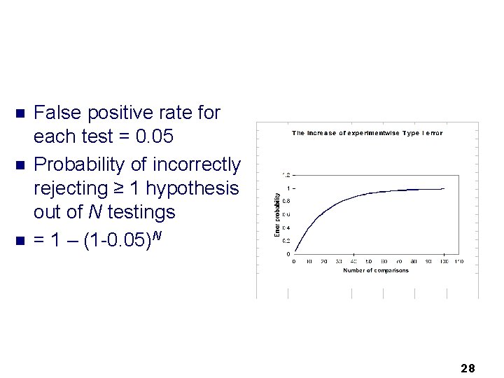
The increase of type I error n It can be shown that when t tests are used to test for differences between multiple groups, the chance of mistakenly declaring significance (Type I Error) is increasing. For example, in the case of 5 groups, if no overall differences exist between any of the groups, using two-sample t tests pair wise, we would have about 30% chance of declaring at least one difference significant, instead of 5% chance. n In general, the t test can be used to test the hypothesis that two group means are not different. To test the hypothesis that three ore more group means are not different, analysis of variance should be used. 27

n n n False positive rate for each test = 0. 05 Probability of incorrectly rejecting ≥ 1 hypothesis out of N testings = 1 – (1 -0. 05)N 28

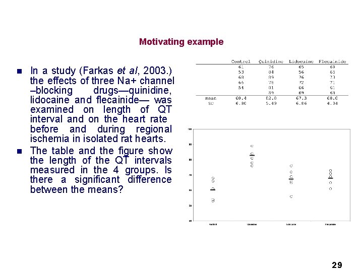
Motivating example n n In a study (Farkas et al, 2003. ) the effects of three Na+ channel –blocking drugs—quinidine, lidocaine and flecainide— was examined on length of QT interval and on the heart rate before and during regional ischemia in isolated rat hearts. The table and the figure show the length of the QT intervals measured in the 4 groups. Is there a significant difference between the means? 29

One-Way ANOVA (Analysis of Variance) Comparison of the mean of several normal populations n Let us suppose that we have t independent samples (t “treatment” groups) drawn from normal populations with equal variances ~N(µi, ). n Assumptions: § Independent samples § normality § Equal variances n Null hypothesis: population means are equal, µ 1=µ 2=. . =µt 30

Method n If the null hypothesis is true, then the populations are the same: they are normal, and they have the same mean and the same variance. This common variance is estimated in two distinct ways: § between-groups variance § within-groups variance n n If the null hypothesis is true, then these two distinct estimates of the variance should be equal ‘New’ (and equivalent) null hypothesis: 2 between= 2 within their equality can be tested by an F ratio test The p-value of this test: § if p>0. 05, then we accept H 0. The analysis is complete. § if p<0. 05, then we reject H 0 at 0. 05 level. There is at least one group-mean different from one of the others 31

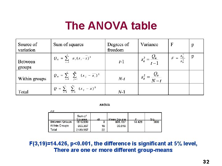
The ANOVA table F(3, 19)=14. 426, p<0. 001, the difference is significant at 5% level, There are one or more different group-means 32

Following-up ANOVA If the F-test of the ANOVA is not significant, we are ready n If the F-test of ANOVA is significant, we might be interested in pairwise comparisons (but t-tests are NOT appropriate!) n 33

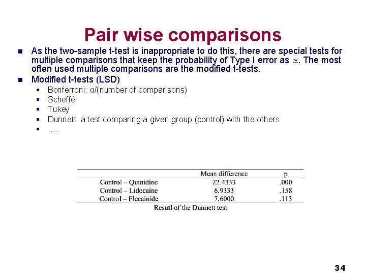
Pair wise comparisons n n As the two-sample t-test is inappropriate to do this, there are special tests for multiple comparisons that keep the probability of Type I error as . The most often used multiple comparisons are the modified t-tests. Modified t-tests (LSD) § § § Bonferroni: α/(number of comparisons) Scheffé Tukey Dunnett: a test comparing a given group (control) with the others …. 34

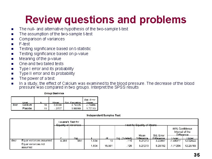
Review questions and problems n n n The null- and alternative hypothesis of the two-sample t-test The assumption of the two-sample t-test Comparison of variances F-test Testing significance based on t-statistic Testing significance based on p-value Meaning of the p-value One-and two tailed tests Type I error and its probability Type II error and its probability The power of a test In a study, the effect of Calcium was examined to the blood pressure. The decrease of the blood pressure was compared in two groups. Interpret the SPSS results 35

Review questions and exercises n n n n One-and two tailed tests The type I error and its probability The type II error and its probability The increase of Type I. error The aim and the nullhypothesis of one-way ANOVA The assumptions of one-way ANOVA The ANOVA table Pair-wise comparisons 36