Highresolution TEM CHAPT ER 28 SUMMARY ANTTI MYLLYNEN

High-resolution TEM CHAPT ER 28 – SUMMARY ANTTI MYLLYNEN

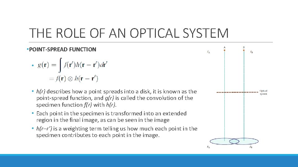
THE ROLE OF AN OPTICAL SYSTEM • POINT-SPREAD FUNCTION • • h(r) describes how a point spreads into a disk, it is known as the point-spread function, and g(r) is called the convolution of the specimen function f(r) with h(r). • Each point in the specimen is transformed into an extended region in the final image, as can be seen in the image • h(r–r’) is a weighting term telling us how much each point in the specimen contributes to each point in the image.

FOURIER TRANSFORM • The intensity of an image at point (x, y) can be expressed with g(x, y) • u = reciprocal lattice vector • G(u) = Fourier transform of g(r) • G(u) can be expressed with Fourier transforms of h(r) and f(r)

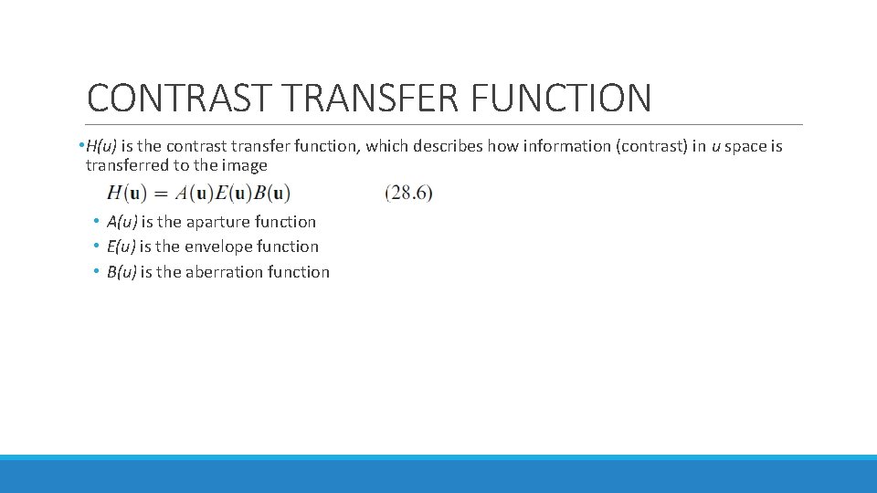
CONTRAST TRANSFER FUNCTION • H(u) is the contrast transfer function, which describes how information (contrast) in u space is transferred to the image • A(u) is the aparture function • E(u) is the envelope function • B(u) is the aberration function

SPATIAL FREQUENCY • High spatial frequencies correspond to large distances from the optic axis in the DP. • The rays which pass through the lens at these large distances are bent through a larger angle by the objective lens. • They are not focused at the same point by the lens, because of spherical aberration, and thus cause a spreading of the point in the image. • The result is that the objective lens magnifies the image but confuses the fine detail. • The resolution we require in HRTEM is limited by this ‘confusion’.

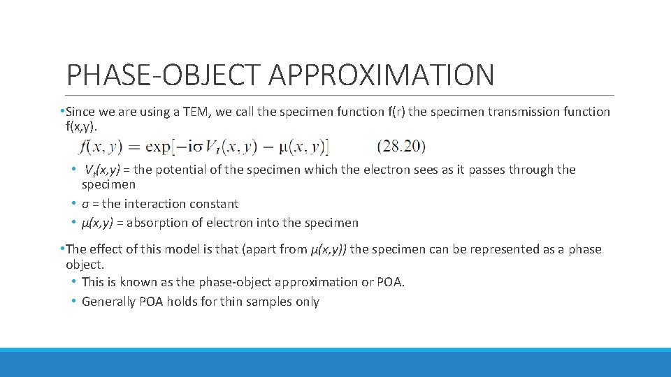
PHASE-OBJECT APPROXIMATION • Since we are using a TEM, we call the specimen function f(r) the specimen transmission function f(x, y). • Vt(x, y) = the potential of the specimen which the electron sees as it passes through the specimen • σ = the interaction constant • μ(x, y) = absorption of electron into the specimen • The effect of this model is that (apart from μ(x, y)) the specimen can be represented as a phase object. • This is known as the phase-object approximation or POA. • Generally POA holds for thin samples only

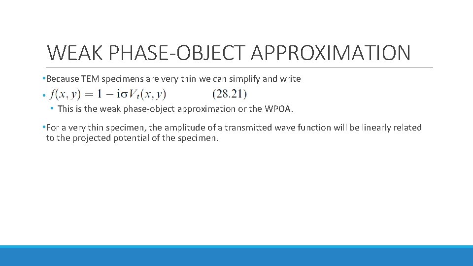
WEAK PHASE-OBJECT APPROXIMATION • Because TEM specimens are very thin we can simplify and write • • This is the weak phase-object approximation or the WPOA. • For a very thin specimen, the amplitude of a transmitted wave function will be linearly related to the projected potential of the specimen.

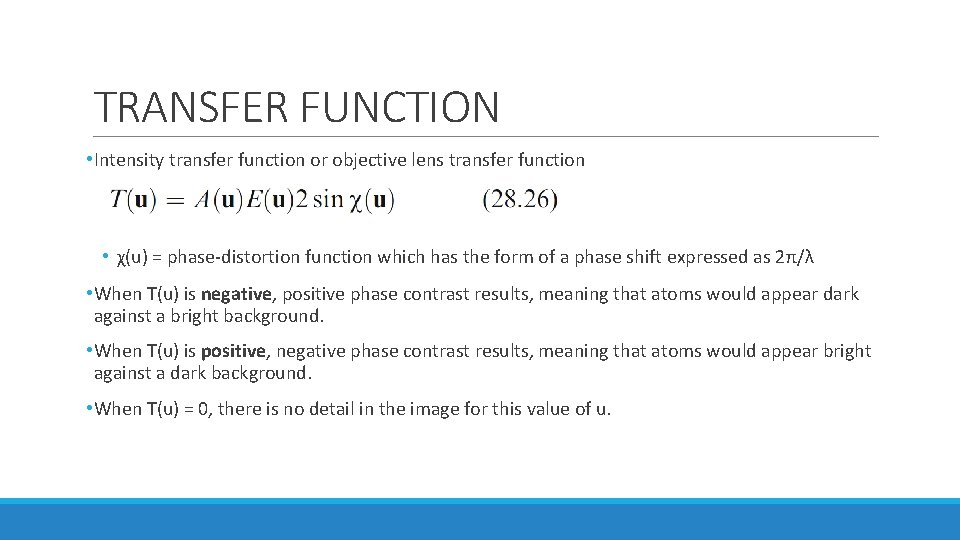
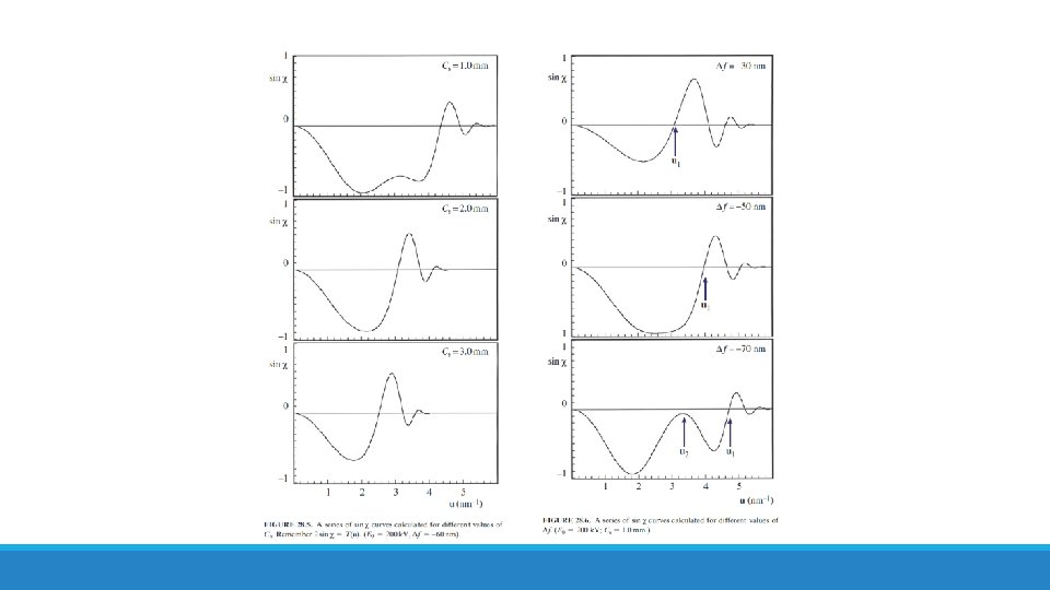
TRANSFER FUNCTION • Intensity transfer function or objective lens transfer function • χ(u) = phase-distortion function which has the form of a phase shift expressed as 2π/λ • When T(u) is negative, positive phase contrast results, meaning that atoms would appear dark against a bright background. • When T(u) is positive, negative phase contrast results, meaning that atoms would appear bright against a dark background. • When T(u) = 0, there is no detail in the image for this value of u.

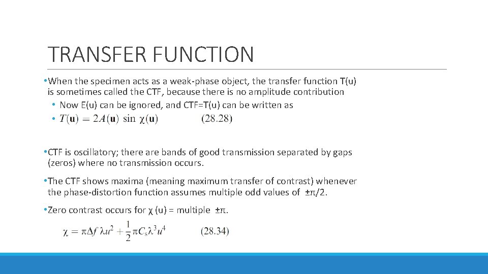
TRANSFER FUNCTION • When the specimen acts as a weak-phase object, the transfer function T(u) is sometimes called the CTF, because there is no amplitude contribution • Now E(u) can be ignored, and CTF=T(u) can be written as • • CTF is oscillatory; there are bands of good transmission separated by gaps (zeros) where no transmission occurs. • The CTF shows maxima (meaning maximum transfer of contrast) whenever the phase-distortion function assumes multiple odd values of ±π/2. • Zero contrast occurs for χ (u) = multiple ±π.

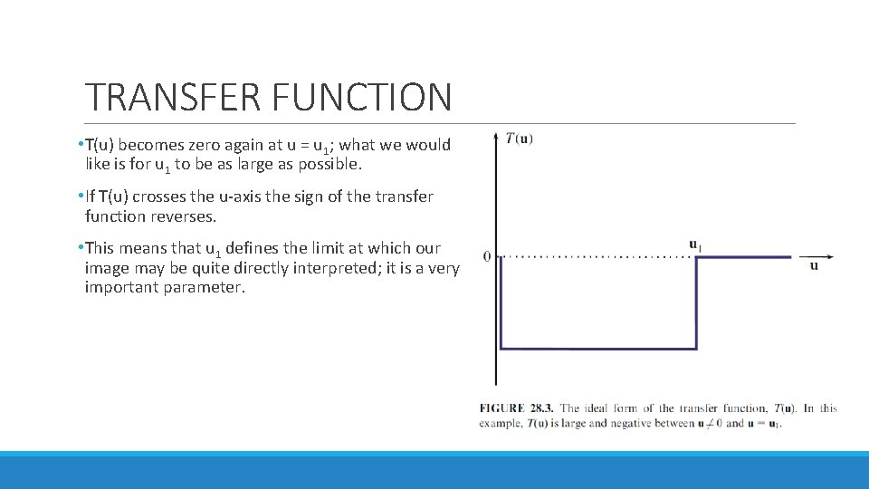
TRANSFER FUNCTION • T(u) becomes zero again at u = u 1; what we would like is for u 1 to be as large as possible. • If T(u) crosses the u-axis the sign of the transfer function reverses. • This means that u 1 defines the limit at which our image may be quite directly interpreted; it is a very important parameter.

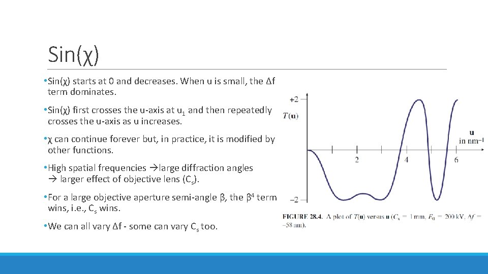
Sin(χ) • Sin(χ) starts at 0 and decreases. When u is small, the Δf term dominates. • Sin(χ) first crosses the u-axis at u 1 and then repeatedly crosses the u-axis as u increases. • χ can continue forever but, in practice, it is modified by other functions. • High spatial frequencies large diffraction angles larger effect of objective lens (Cs). • For a large objective aperture semi-angle β, the β 4 term wins, i. e. , Cs wins. • We can all vary Δf - some can vary Cs too.

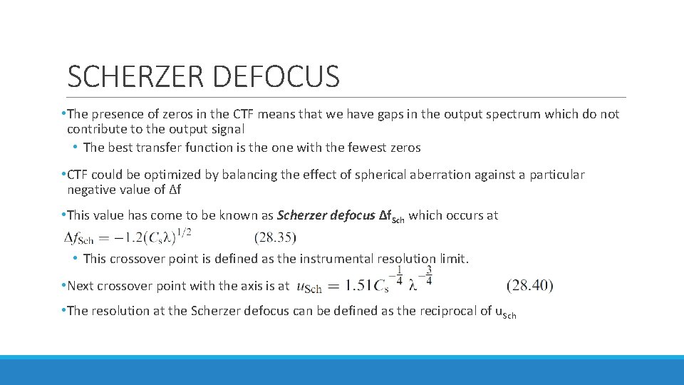
SCHERZER DEFOCUS • The presence of zeros in the CTF means that we have gaps in the output spectrum which do not contribute to the output signal • The best transfer function is the one with the fewest zeros • CTF could be optimized by balancing the effect of spherical aberration against a particular negative value of Δf • This value has come to be known as Scherzer defocus Δf. Sch which occurs at • This crossover point is defined as the instrumental resolution limit. • Next crossover point with the axis is at • The resolution at the Scherzer defocus can be defined as the reciprocal of u. Sch

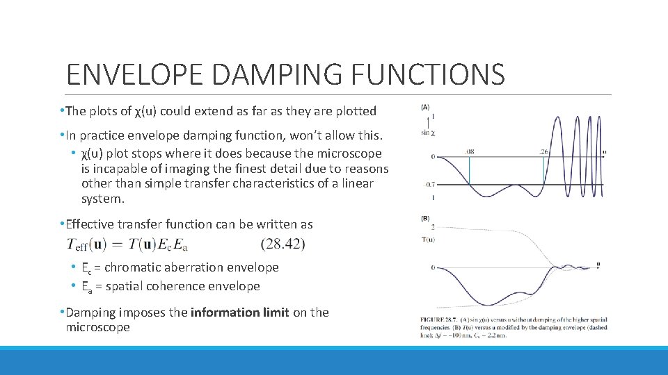
ENVELOPE DAMPING FUNCTIONS • The plots of χ(u) could extend as far as they are plotted • In practice envelope damping function, won’t allow this. • χ(u) plot stops where it does because the microscope is incapable of imaging the finest detail due to reasons other than simple transfer characteristics of a linear system. • Effective transfer function can be written as • Ec = chromatic aberration envelope • Ea = spatial coherence envelope • Damping imposes the information limit on the microscope

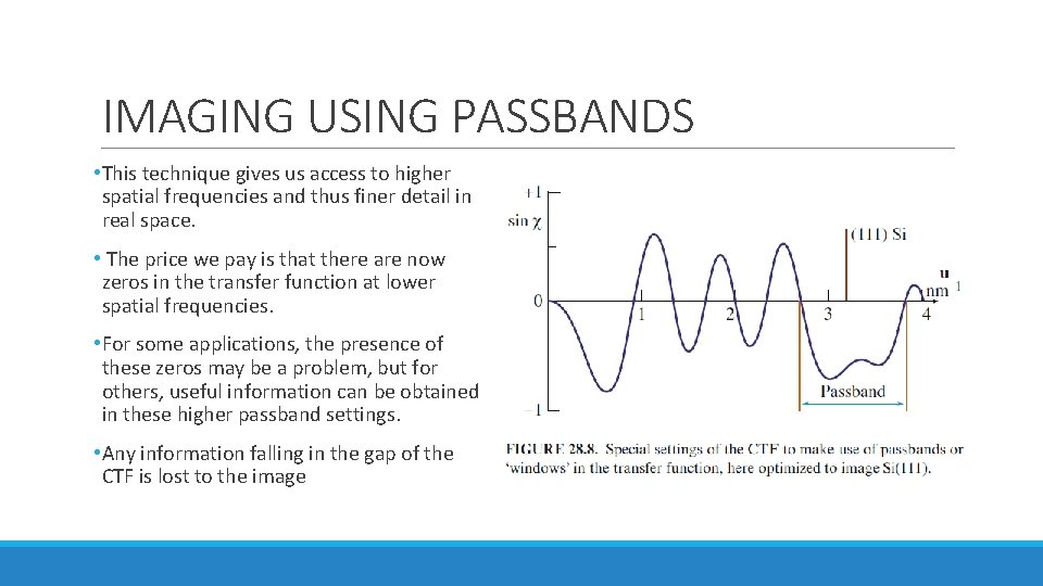
IMAGING USING PASSBANDS • This technique gives us access to higher spatial frequencies and thus finer detail in real space. • The price we pay is that there are now zeros in the transfer function at lower spatial frequencies. • For some applications, the presence of these zeros may be a problem, but for others, useful information can be obtained in these higher passband settings. • Any information falling in the gap of the CTF is lost to the image

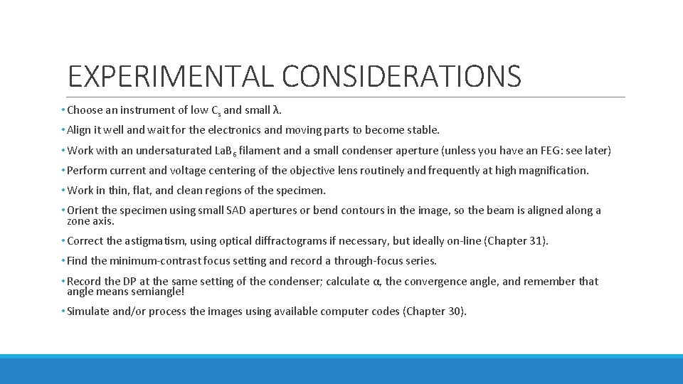
EXPERIMENTAL CONSIDERATIONS • Choose an instrument of low Cs and small λ. • Align it well and wait for the electronics and moving parts to become stable. • Work with an undersaturated La. B 6 filament and a small condenser aperture (unless you have an FEG: see later) • Perform current and voltage centering of the objective lens routinely and frequently at high magnification. • Work in thin, flat, and clean regions of the specimen. • Orient the specimen using small SAD apertures or bend contours in the image, so the beam is aligned along a zone axis. • Correct the astigmatism, using optical diffractograms if necessary, but ideally on-line (Chapter 31). • Find the minimum-contrast focus setting and record a through-focus series. • Record the DP at the same setting of the condenser; calculate α, the convergence angle, and remember that angle means semiangle! • Simulate and/or process the images using available computer codes (Chapter 30).

COMA • If a point object on the optic axis is imaged as a point, a similar point object off the axis may appear distorted. • This distortion is known as coma or comatic aberration.

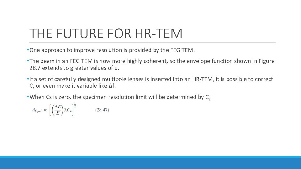
THE FUTURE FOR HR-TEM • One approach to improve resolution is provided by the FEG TEM. • The beam in an FEG TEM is now more highly coherent, so the envelope function shown in Figure 28. 7 extends to greater values of u. • If a set of carefully designed multipole lenses is inserted into an HR-TEM, it is possible to correct Cs or even make it variable like Δf. • When Cs is zero, the specimen resolution limit will be determined by Cc

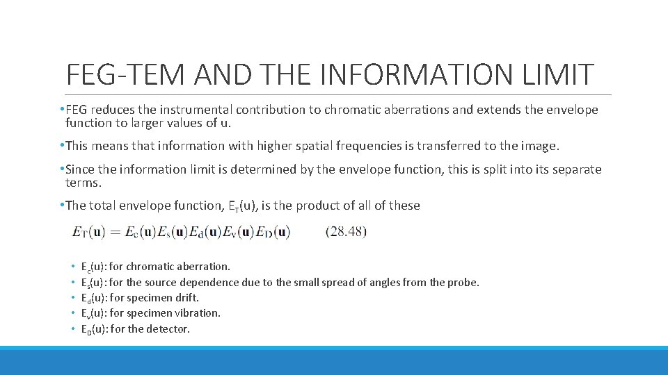
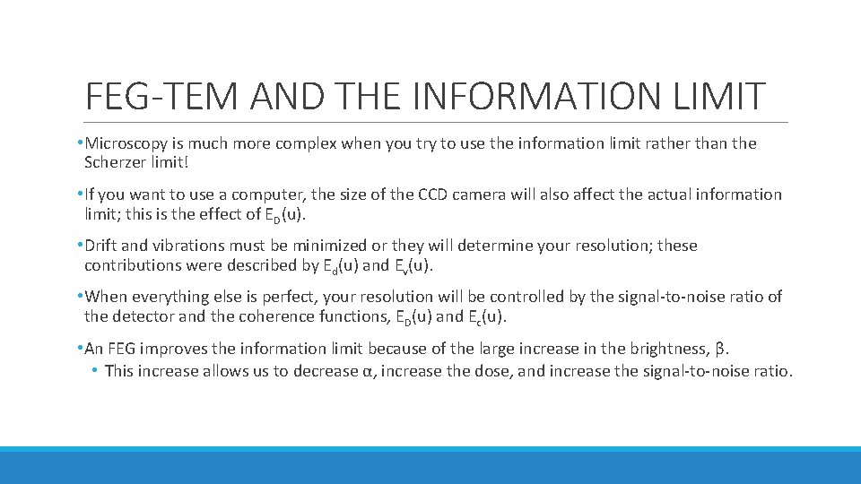
FEG-TEM AND THE INFORMATION LIMIT • FEG reduces the instrumental contribution to chromatic aberrations and extends the envelope function to larger values of u. • This means that information with higher spatial frequencies is transferred to the image. • Since the information limit is determined by the envelope function, this is split into its separate terms. • The total envelope function, ET(u), is the product of all of these • • • Ec(u): for chromatic aberration. Es(u): for the source dependence due to the small spread of angles from the probe. Ed(u): for specimen drift. Ev(u): for specimen vibration. ED(u): for the detector.

FEG-TEM AND THE INFORMATION LIMIT • Microscopy is much more complex when you try to use the information limit rather than the Scherzer limit! • If you want to use a computer, the size of the CCD camera will also affect the actual information limit; this is the effect of ED(u). • Drift and vibrations must be minimized or they will determine your resolution; these contributions were described by Ed(u) and Ev(u). • When everything else is perfect, your resolution will be controlled by the signal-to-noise ratio of the detector and the coherence functions, ED(u) and Ec(u). • An FEG improves the information limit because of the large increase in the brightness, β. • This increase allows us to decrease α, increase the dose, and increase the signal-to-noise ratio.

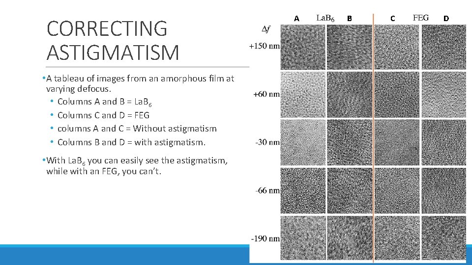
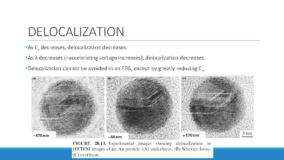
PROBLEMS WHEN USING FEG • A cold FEG (CFEG) allows us to extract a very high current per unit area, but the total area of the emitting region is very small so that the extraction current is <5 n. A. • This current can be increased if we thermally assist the field emission by heating the Schottky emitter to 1500°C 10 x bigger source diameter with decreasing spatial coherency and larger energy spread • Correcting astigmatism is very tricky with an FEG if compared to La. B 6 • Image on the next slide • Focal series of images are a challenge, because you can now use a very large range of Δf • Determining the value of the Δf can be challenging • Image delocalization occurs when detail in the image is displaced relative to its true location in the specimen.

CORRECTING ASTIGMATISM • A tableau of images from an amorphous film at varying defocus. • Columns A and B = La. B 6 • Columns C and D = FEG • columns A and C = Without astigmatism • Columns B and D = with astigmatism. • With La. B 6 you can easily see the astigmatism, while with an FEG, you can’t. A B C D

DELOCALIZATION • As Cs decreases, delocalization decreases. • As λ decreases (=accelerating voltage increases), delocalization decreases. • Delocalization cannot be avoided in an FEG, except by greatly reducing Cs.

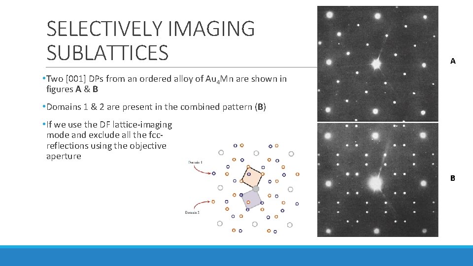
SELECTIVELY IMAGING SUBLATTICES A • Two [001] DPs from an ordered alloy of Au 4 Mn are shown in figures A & B • Domains 1 & 2 are present in the combined pattern (B) • If we use the DF lattice-imaging mode and exclude all the fccreflections using the objective aperture B

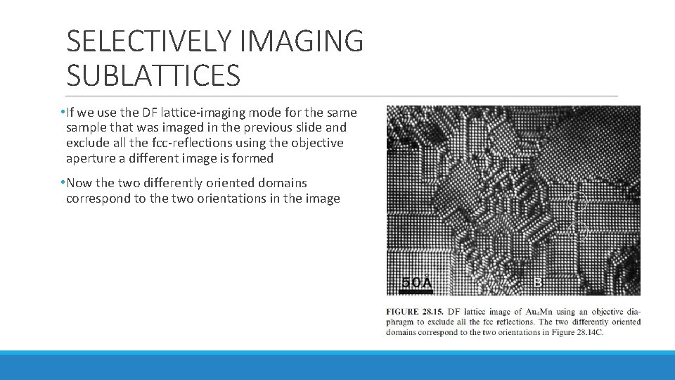
SELECTIVELY IMAGING SUBLATTICES • If we use the DF lattice-imaging mode for the sample that was imaged in the previous slide and exclude all the fcc-reflections using the objective aperture a different image is formed • Now the two differently oriented domains correspond to the two orientations in the image

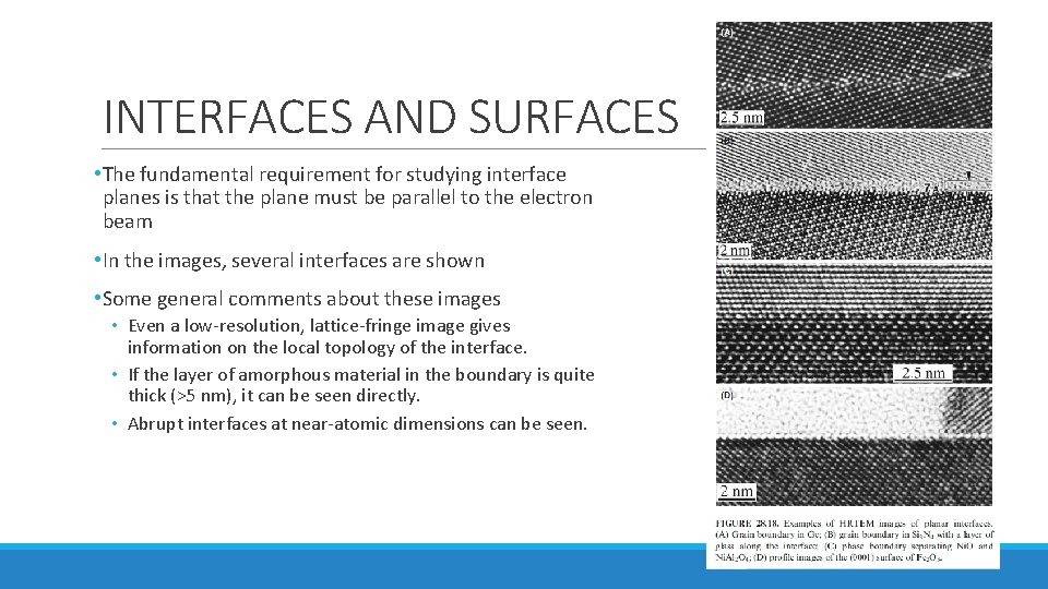
INTERFACES AND SURFACES • The fundamental requirement for studying interface planes is that the plane must be parallel to the electron beam • In the images, several interfaces are shown • Some general comments about these images • Even a low-resolution, lattice-fringe image gives information on the local topology of the interface. • If the layer of amorphous material in the boundary is quite thick (>5 nm), it can be seen directly. • Abrupt interfaces at near-atomic dimensions can be seen.

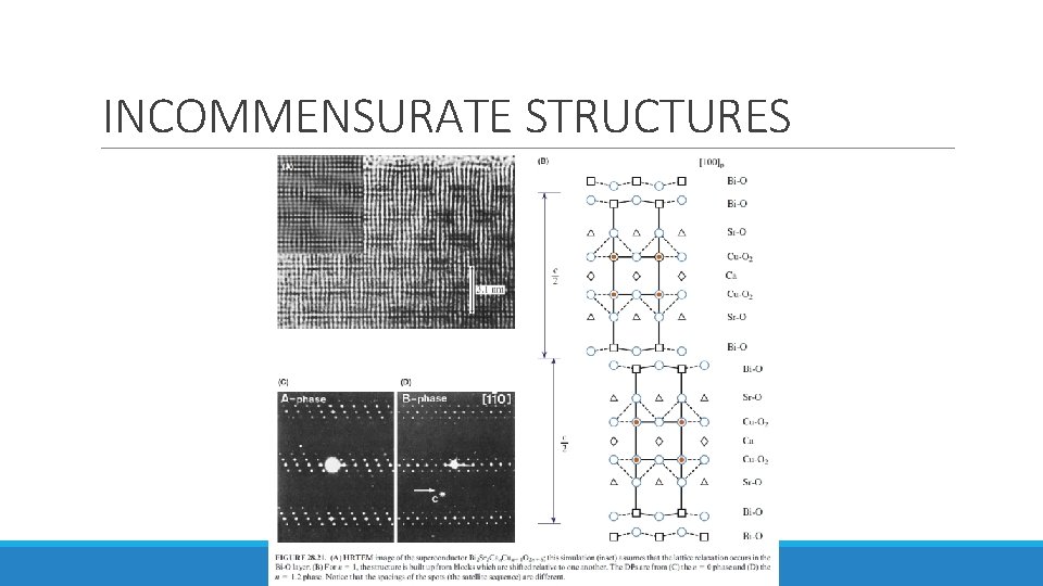
INCOMMENSURATE STRUCTURES • Three different types of incommensurate (modulated) structures: 1. Periodic modules of the parent structure separated by interfaces • The interface may be a stacking fault (SF), twin boundary (TB), anti-phase boundary (APB), inversion domain boundary (IDB), crystallographic shear (CS) plane, or discommensuration wall. 2. The interface may be a stacking fault (SF), twin boundary (TB), anti-phase boundary (APB), inversion domain boundary (IDB), crystallographic shear (CS) plane, or discommensuration wall. 3. Images of this structure produced with the beam along the orthogonal direction would be difficult to explain.

INCOMMENSURATE STRUCTURES

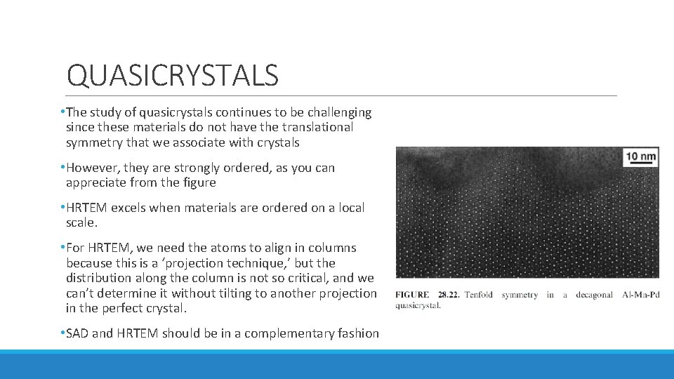
QUASICRYSTALS • The study of quasicrystals continues to be challenging since these materials do not have the translational symmetry that we associate with crystals • However, they are strongly ordered, as you can appreciate from the figure • HRTEM excels when materials are ordered on a local scale. • For HRTEM, we need the atoms to align in columns because this is a ‘projection technique, ’ but the distribution along the column is not so critical, and we can’t determine it without tilting to another projection in the perfect crystal. • SAD and HRTEM should be in a complementary fashion

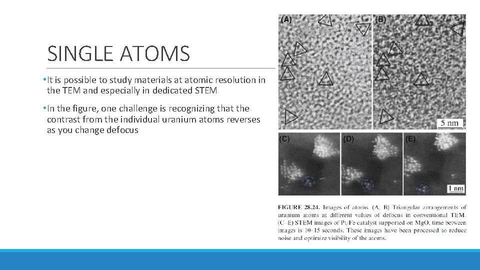
SINGLE ATOMS • It is possible to study materials at atomic resolution in the TEM and especially in dedicated STEM • In the figure, one challenge is recognizing that the contrast from the individual uranium atoms reverses as you change defocus