Hidden Markov Models Yves Moreau Katholieke Universiteit Leuven

Hidden Markov Models Yves Moreau Katholieke Universiteit Leuven

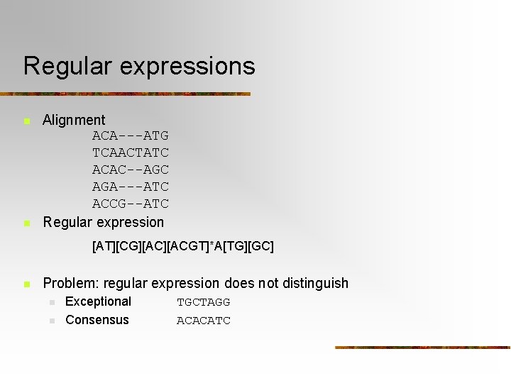
Regular expressions n n Alignment ACA---ATG TCAACTATC ACAC--AGC AGA---ATC ACCG--ATC Regular expression [AT][CG][ACGT]*A[TG][GC] n Problem: regular expression does not distinguish n n Exceptional Consensus TGCTAGG ACACATC

Hidden Markov Models Sequence score Transition probabilities . 4 A C G T Emission probabilities . 2. 4. 2. 2 . 6 A C G T . 8 0 0. 2 1. 0 A C G T 0. 8. 2 0 1. 0 A C G T . 8. 2 0 0 . 4 A C G T 1 0 0 0 1. 0 A C G T 0 0. 2. 8 1. 0 A C G T 0. 8. 2 0

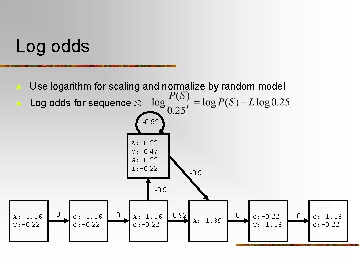
Log odds n Use logarithm for scaling and normalize by random model n Log odds for sequence S: -0. 92 A: -0. 22 C: 0. 47 G: -0. 22 T: -0. 22 -0. 51 A: 1. 16 T: -0. 22 0 C: 1. 16 G: -0. 22 0 A: 1. 16 C: -0. 22 -0. 92 A: 1. 39 0 G: -0. 22 T: 1. 16 0 C: 1. 16 G: -0. 22

Log odds Sequence Log odds ACAC--ATC (consensus) 6. 7 ACA---ATG 4. 9 TCAACTATC 3. 0 ACAC--AGC 5. 3 AGA---ATC 4. 9 ACCG--ATC 4. 6 TGCT--AGG (exceptional) -0. 97

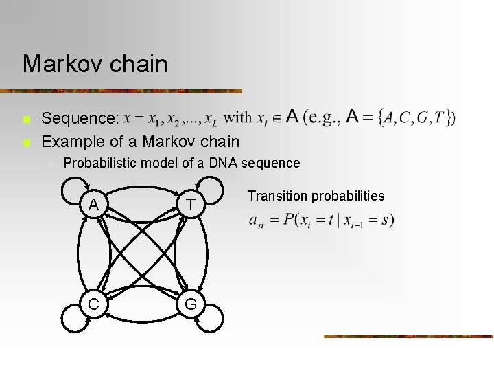
Markov chain n n Sequence: Example of a Markov chain n Probabilistic model of a DNA sequence A T C G Transition probabilities

Markov property n Probability of a sequence through Bayes’ rule n Markov property n “The future is only function of the present and not of the past”

Beginning and end of a sequence n n Computation of the probability is not homogeneous Length distribution is not modeled n n P(length=L) unspecified Solution n Modeling of beginning and end of the sequence A a w C n The probability to observe a sequence of a given length decreases with the length of the sequence T G

Hidden Markov Models Sequence score Transition probabilities . 4 A C G T Emission probabilities . 2. 4. 2. 2 . 6 A C G T . 8 0 0. 2 1. 0 A C G T 0. 8. 2 0 1. 0 A C G T . 8. 2 0 0 . 4 A C G T 1 0 0 0 1. 0 A C G T 0 0. 2. 8 1. 0 A C G T 0. 8. 2 0

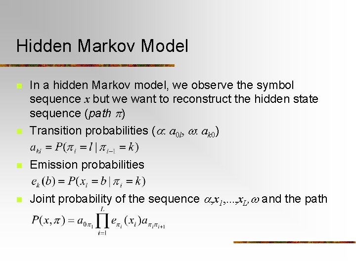
Hidden Markov Model n In a hidden Markov model, we observe the symbol sequence x but we want to reconstruct the hidden state sequence (path p) Transition probabilities (a: a 0 l, w: ak 0) n Emission probabilities n Joint probability of the sequence a, x 1, . . . , x. L, w and the path n

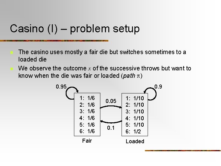
Casino (I) – problem setup n n The casino uses mostly a fair die but switches sometimes to a loaded die We observe the outcome x of the successive throws but want to know when the die was fair or loaded (path p) 0. 95 1: 2: 3: 4: 5: 6: 1/6 1/6 1/6 Fair 0. 05 0. 1 1: 2: 3: 4: 5: 6: 1/10 1/10 1/2 Loaded

Estimation of the sequence and state probabilities

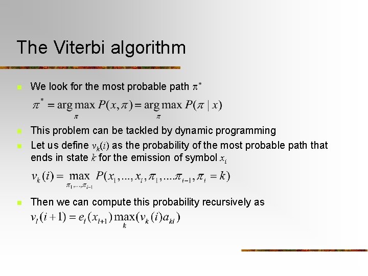
The Viterbi algorithm n We look for the most probable path p* n n This problem can be tackled by dynamic programming Let us define vk(i) as the probability of the most probable path that ends in state k for the emission of symbol xi n Then we can compute this probability recursively as

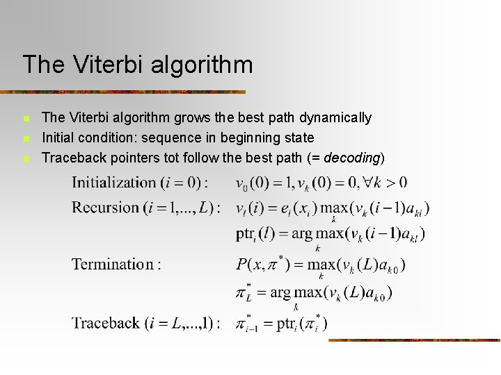
The Viterbi algorithm n n n The Viterbi algorithm grows the best path dynamically Initial condition: sequence in beginning state Traceback pointers tot follow the best path (= decoding)

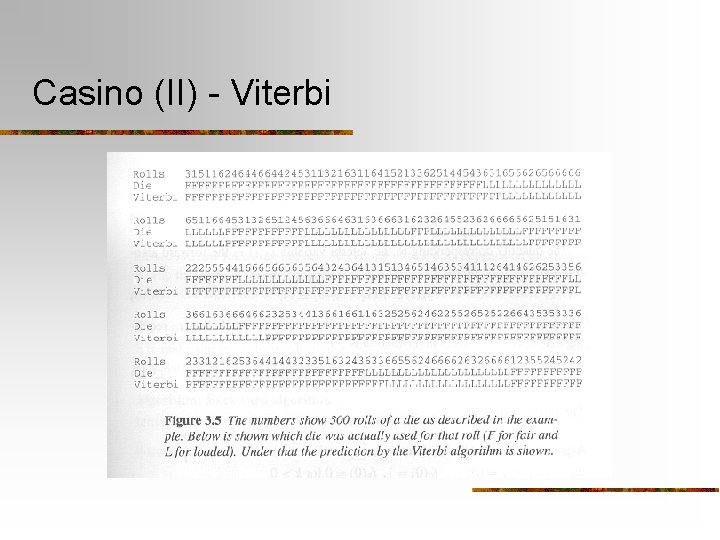
Casino (II) - Viterbi

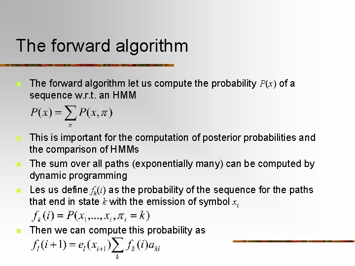
The forward algorithm n The forward algorithm let us compute the probability P(x) of a sequence w. r. t. an HMM n This is important for the computation of posterior probabilities and the comparison of HMMs The sum over all paths (exponentially many) can be computed by dynamic programming Les us define fk(i) as the probability of the sequence for the paths that end in state k with the emission of symbol xi n n n Then we can compute this probability as

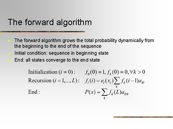
The forward algorithm n n n The forward algorithm grows the total probability dynamically from the beginning to the end of the sequence Initial condition: sequence in beginning state End: all states converge to the end state

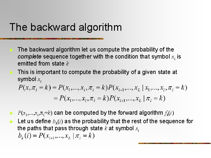
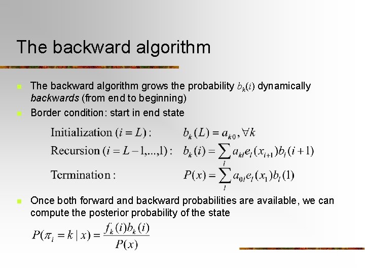
The backward algorithm n n The backward algorithm let us compute the probability of the complete sequence together with the condition that symbol xi is emitted from state k This is important to compute the probability of a given state at symbol xi P(x 1, . . . , xi, pi=k) can be computed by the forward algorithm fk(i) Let us define bk(i) as the probability that the rest of the sequence for the paths that pass through state k at symbol xi

The backward algorithm n n n The backward algorithm grows the probability bk(i) dynamically backwards (from end to beginning) Border condition: start in end state Once both forward and backward probabilities are available, we can compute the posterior probability of the state

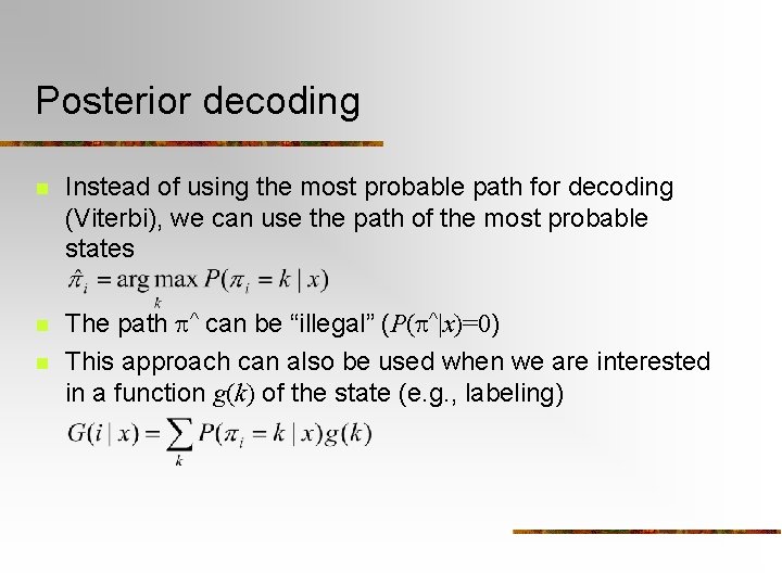
Posterior decoding n Instead of using the most probable path for decoding (Viterbi), we can use the path of the most probable states n The path p^ can be “illegal” (P(p^|x)=0) This approach can also be used when we are interested in a function g(k) of the state (e. g. , labeling) n

Casino (III) – posterior decodering n Posterior probability of the state “fair” w. r. t. the die throws

Casino (IV) – posterior decodering n n New situation : P(xi+1 = FAIR | xi = FAIR) = 0. 99 Viterbi decoding cannot detect the cheating from 1000 throws, while posterior decoding does 0. 99 1: 2: 3: 4: 5: 6: 1/6 1/6 1/6 Fair 0. 01 0. 1 1: 2: 3: 4: 5: 6: 1/10 1/10 1/2 Loaded

Parameter estimation for HMMs

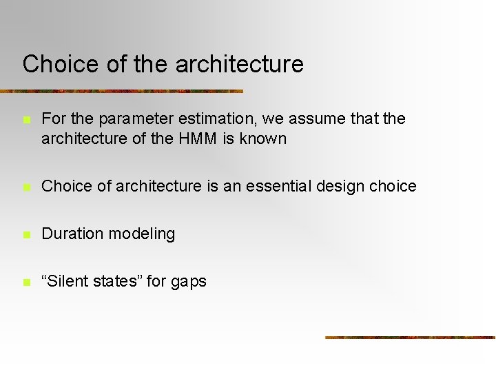
Choice of the architecture n For the parameter estimation, we assume that the architecture of the HMM is known n Choice of architecture is an essential design choice n Duration modeling n “Silent states” for gaps

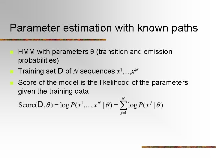
Parameter estimation with known paths n HMM with parameters q (transition and emission probabilities) n Training set D of N sequences x 1, . . . , x. N n Score of the model is the likelihood of the parameters given the training data

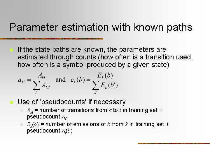
Parameter estimation with known paths n If the state paths are known, the parameters are estimated through counts (how often is a transition used, how often is a symbol produced by a given state) n Use of ‘pseudocounts’ if necessary n n Akl = number of transitions from k to l in training set + pseudocount rkl Ek(b) = number of emissions of b from k in training set + pseudocount rk(b)

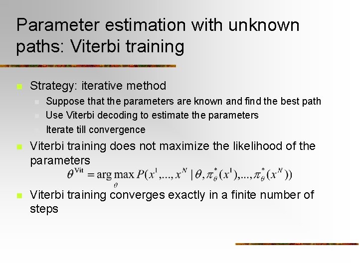
Parameter estimation with unknown paths: Viterbi training n Strategy: iterative method n n n Suppose that the parameters are known and find the best path Use Viterbi decoding to estimate the parameters Iterate till convergence n Viterbi training does not maximize the likelihood of the parameters n Viterbi training converges exactly in a finite number of steps

Parameter estimation with unknown paths: Baum-Welch training n Strategy: parallel to Viterbi but we use the expected value for the transition and emission counts (instead of using only the best path) n For the transitions n For the emissions

Parameter estimation with unknown paths: Baum-Welch training n n Initialization: Choose arbitrary model parameters Recursion: n n Set all transitions and emission variables to their pseudocount For all sequences j = 1, . . . , n n n n Compute fk(i) for sequence j with the forward algorithm Compute bk(i) for sequence j with the backward algorithm Add the contributions to A and E Compute the new model parameters akl =Akl/SAkl’ and ek(b) Compute the log-likelihood of the model End: stop when the log-likelihood does not change more than by some threshold or when the maximum number of iterations is exceeded

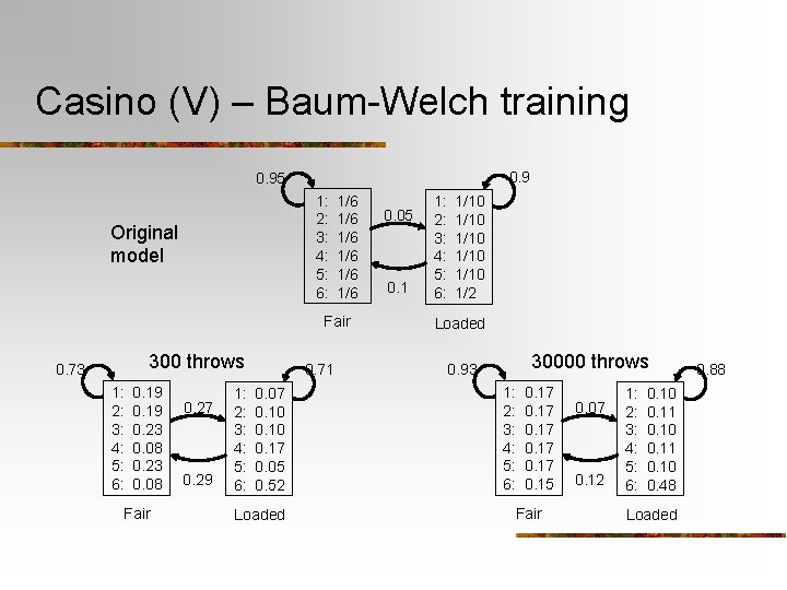
Casino (V) – Baum-Welch training 0. 95 1: 2: 3: 4: 5: 6: Original model 1/6 1/6 1/6 Fair 300 throws 0. 73 1: 2: 3: 4: 5: 6: 0. 19 0. 23 0. 08 Fair 0. 27 0. 29 1: 2: 3: 4: 5: 6: 0. 71 0. 07 0. 10 0. 17 0. 05 0. 52 Loaded 0. 05 0. 1 1: 2: 3: 4: 5: 6: 1/10 1/10 1/2 Loaded 30000 throws 0. 93 1: 2: 3: 4: 5: 6: 0. 17 0. 15 Fair 0. 07 0. 12 1: 2: 3: 4: 5: 6: 0. 10 0. 11 0. 10 0. 48 Loaded 0. 88

Numerical stability n n Many expressions contain products of many probabilities This causes underflow when we compute these expressions For Viterbi, this can be solved by working with the logarithms For the forward and backward algorithms, we can work with an approximation to the logarithm or by working with rescaled variables

Summary n n Hidden Markov Models Computation of sequence and state probabilities n n Viterbi computation of the best state path The forward algorithm for the computation of the probability of a sequence The backward algorithm for the computation of state probabilities Parameter estimation for HMMs n n Parameter estimation with known paths Parameter estimation with unknown paths n n Viterbi training Baum-Welch training