Getting the Most out of Your Sample Edith

Getting the Most out of Your Sample Edith Cohen Haim Kaplan Tel Aviv University

Why data is sampled • Lots of Data: measurements, Web searches, tweets, downloads, locations, content, social networks, and all this both historic and current… • To get value from data we need to be able to process queries over it • But resources are constrained: Data too large to: transmit, store in full, to process even if stored in full…

Random samples • A compact synopsis/summary of the data. Easier to store, transmit, update, and manipulate • Aggregate queries over the data can be approximately (and efficiently) answered from the sample • Flexible: Same sample supports many types of queries (which do not have to be known in advance)

Queries and estimators The value of our sampled data hinges on the quality of our estimators • Estimation of some basic (sub)population statistics is well understood (sample mean, variance, …) • We need to better understand how to estimate other basic queries: – difference norms (anomaly/change detection) – distinct counts

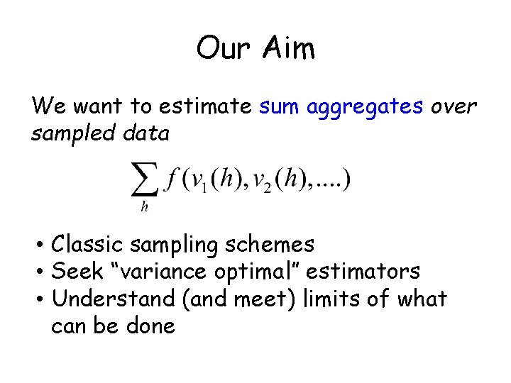
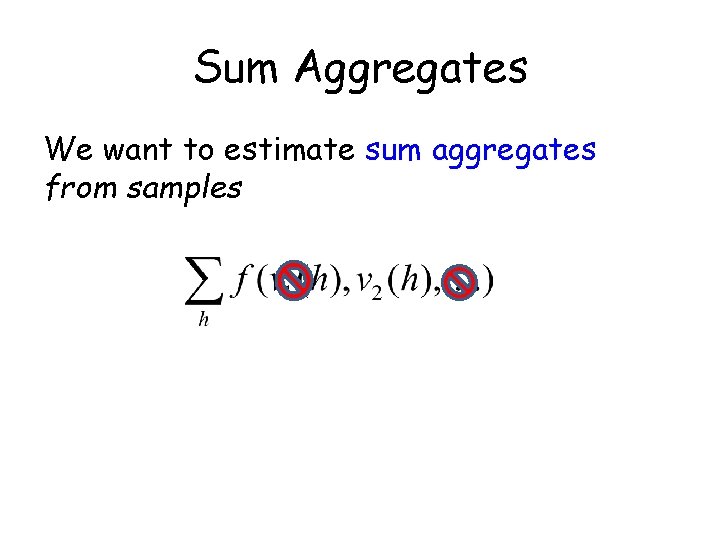
Our Aim We want to estimate sum aggregates over sampled data • Classic sampling schemes • Seek “variance optimal” estimators • Understand (and meet) limits of what can be done

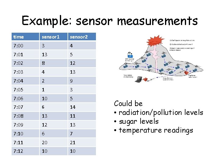
Example: sensor measurements time sensor 1 sensor 2 7: 00 3 4 7: 01 13 5 7: 02 8 12 7: 03 4 13 7: 04 2 9 7: 05 1 3 7: 06 10 5 7: 07 6 14 7: 08 13 11 7: 09 12 13 7: 10 6 7 7: 11 20 21 7: 12 10 10 Could be • radiation/pollution levels • sugar levels • temperature readings

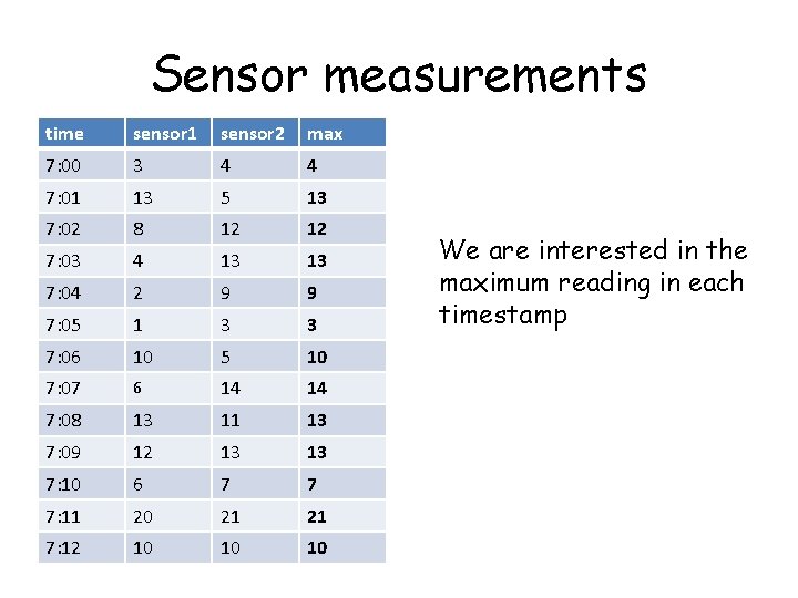
Sensor measurements time sensor 1 sensor 2 max 7: 00 3 4 4 7: 01 13 5 13 7: 02 8 12 12 7: 03 4 13 13 7: 04 2 9 9 7: 05 1 3 3 7: 06 10 5 10 7: 07 6 14 14 7: 08 13 11 13 7: 09 12 13 13 7: 10 6 7 7 7: 11 20 21 21 7: 12 10 10 10 We are interested in the maximum reading in each timestamp

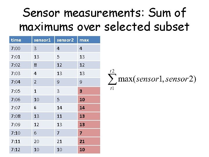
Sensor measurements: Sum of maximums over selected subset time sensor 1 sensor 2 max 7: 00 3 4 4 7: 01 13 5 13 7: 02 8 12 12 7: 03 4 13 13 7: 04 2 9 9 7: 05 1 3 3 7: 06 10 5 10 7: 07 6 14 14 7: 08 13 11 13 7: 09 12 13 13 7: 10 6 7 7 7: 11 20 21 21 7: 12 10 10 10

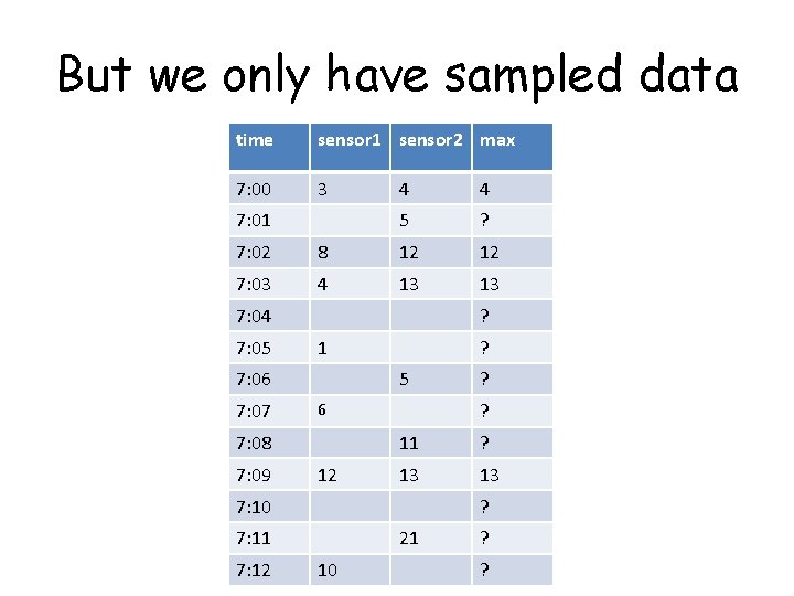
But we only have sampled data time sensor 1 sensor 2 max 7: 00 3 7: 01 4 4 5 ? 7: 02 8 12 12 7: 03 4 13 13 7: 04 7: 05 ? 1 7: 06 7: 07 5 12 11 ? 13 13 7: 10 ? 7: 11 7: 12 ? ? 6 7: 08 7: 09 ? 21 10 ? ?

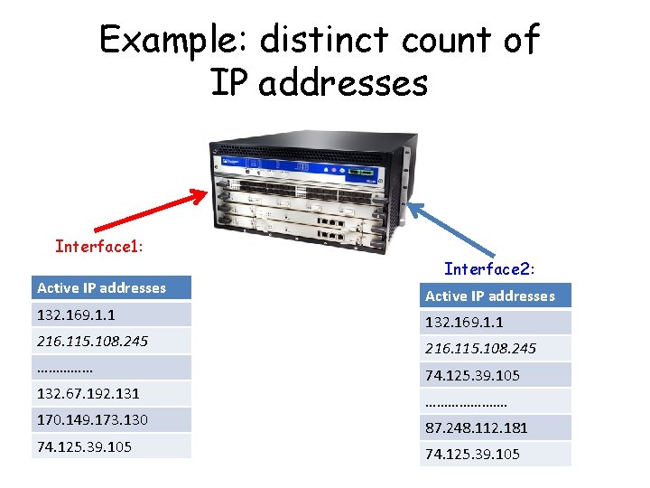
Example: distinct count of IP addresses Interface 1: Active IP addresses 132. 169. 1. 1 216. 115. 108. 245 …………… 132. 67. 192. 131 170. 149. 173. 130 74. 125. 39. 105 Interface 2: Active IP addresses 132. 169. 1. 1 216. 115. 108. 245 74. 125. 39. 105 …………………. 87. 248. 112. 181 74. 125. 39. 105

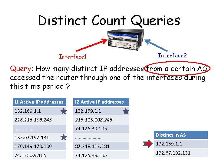
Distinct Count Queries Interface 1 Interface 2 Query: How many distinct IP addresses from a certain AS accessed the router through one of the interfaces during this time period ? I 1 Active IP addresses I 2 Active IP addresses 132. 169. 1. 1 216. 115. 108. 245 …………… 74. 125. 39. 105 132. 67. 192. 131 …………………. 170. 149. 173. 130 87. 248. 112. 181 74. 125. 39. 105 Distinct in AS 132. 169. 1. 1 132. 67. 192. 131

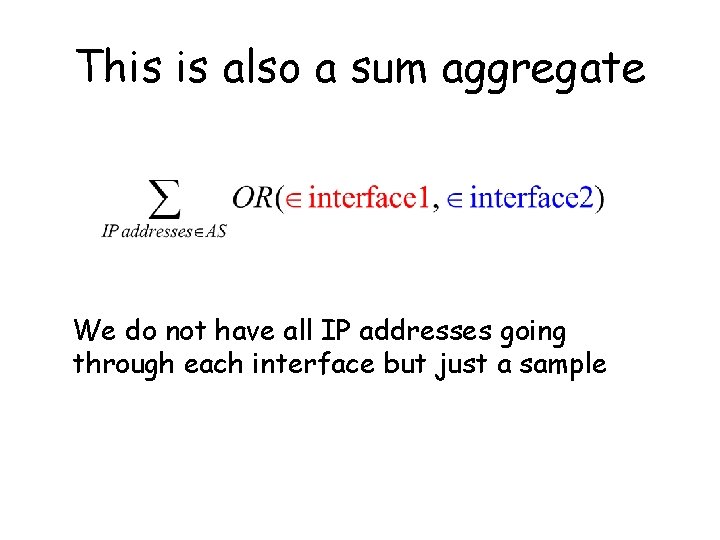
This is also a sum aggregate We do not have all IP addresses going through each interface but just a sample

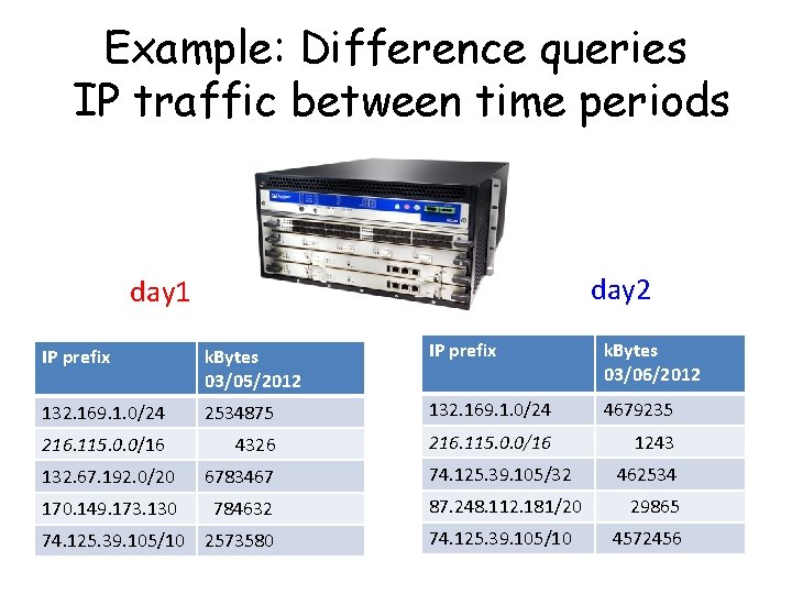
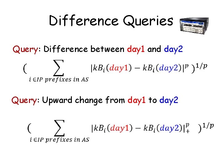
Example: Difference queries IP traffic between time periods day 2 day 1 IP prefix k. Bytes 03/05/2012 IP prefix k. Bytes 03/06/2012 132. 169. 1. 0/24 2534875 132. 169. 1. 0/24 4679235 216. 115. 0. 0/16 4326 216. 115. 0. 0/16 1243 132. 67. 192. 0/20 6783467 74. 125. 39. 105/32 462534 170. 149. 173. 130 784632 87. 248. 112. 181/20 29865 74. 125. 39. 105/10 4572456 74. 125. 39. 105/10 2573580

Difference Queries Query: Difference between day 1 and day 2 Query: Upward change from day 1 to day 2

Sum Aggregates We want to estimate sum aggregates from samples

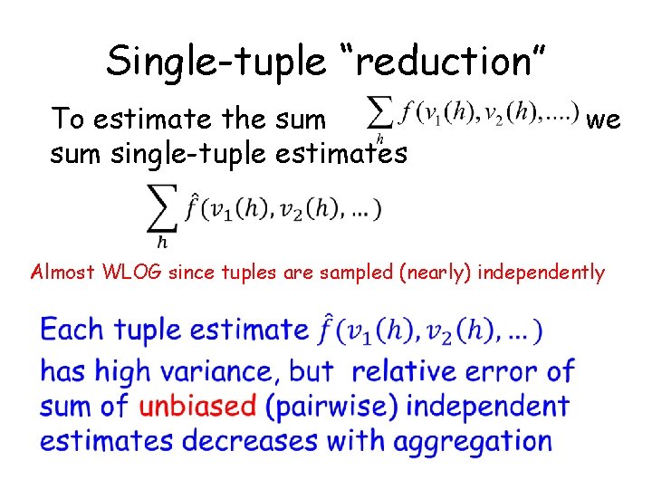
Single-tuple “reduction” To estimate the sum single-tuple estimates we Almost WLOG since tuples are sampled (nearly) independently

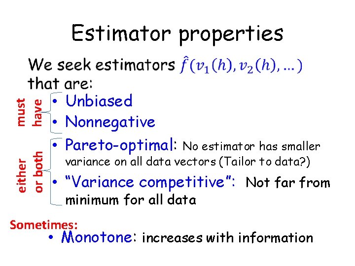
Estimator properties either or both must have • Unbiased • Nonnegative • Pareto-optimal: No estimator has smaller variance on all data vectors (Tailor to data? ) • “Variance competitive”: Not far from minimum for all data Sometimes: • Monotone: increases with information

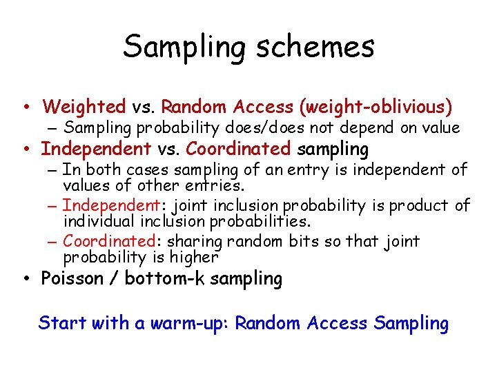
Sampling schemes • Weighted vs. Random Access (weight-oblivious) – Sampling probability does/does not depend on value • Independent vs. Coordinated sampling – In both cases sampling of an entry is independent of values of other entries. – Independent: joint inclusion probability is product of individual inclusion probabilities. – Coordinated: sharing random bits so that joint probability is higher • Poisson / bottom-k sampling Start with a warm-up: Random Access Sampling

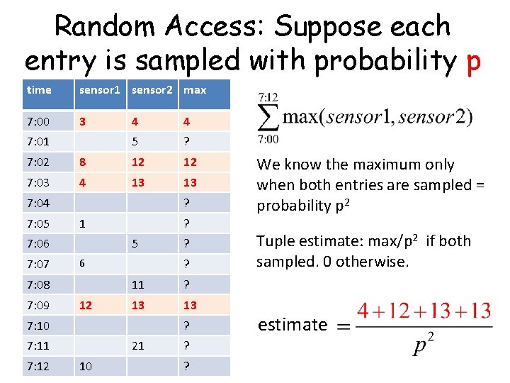
Random Access: Suppose each entry is sampled with probability p time sensor 1 sensor 2 max 7: 00 3 7: 01 4 4 5 ? 7: 02 8 12 12 7: 03 4 13 13 7: 04 7: 05 ? 1 7: 06 7: 07 5 12 11 ? 13 13 7: 10 ? 7: 11 7: 12 ? ? 6 7: 08 7: 09 ? 21 10 ? ? We know the maximum only when both entries are sampled = probability p 2 Tuple estimate: max/p 2 if both sampled. 0 otherwise. estimate

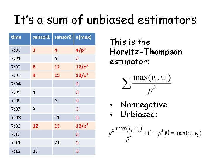
It’s a sum of unbiased estimators time sensor 1 sensor 2 e(max) 7: 00 3 7: 01 4 4/p 2 5 0 7: 02 8 12 12/p 2 7: 03 4 13 13/p 2 7: 04 7: 05 0 1 7: 06 7: 07 0 5 12 11 0 13 13/p 2 7: 10 0 7: 11 7: 12 0 0 6 7: 08 7: 09 This is the Horvitz-Thompson estimator: 21 10 0 0 • Nonnegative • Unbiased:

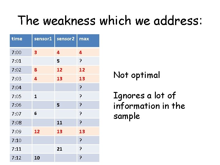
The weakness which we address: time sensor 1 sensor 2 max 7: 00 3 7: 01 4 4 5 ? 7: 02 8 12 12 7: 03 4 13 13 7: 04 7: 05 ? 1 7: 06 7: 07 5 12 11 ? 13 13 7: 10 ? 7: 11 7: 12 ? ? 6 7: 08 7: 09 ? 21 10 ? ? Not optimal Ignores a lot of information in the sample

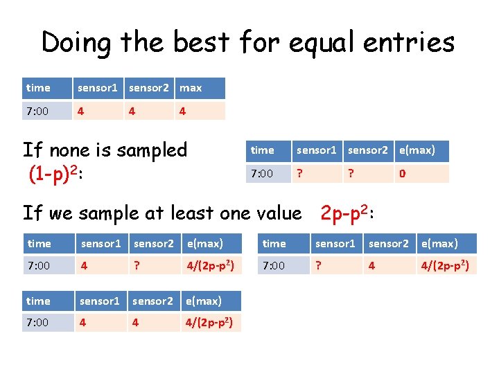
Doing the best for equal entries time sensor 1 sensor 2 max 7: 00 4 4 4 If none is sampled (1 -p)2: time sensor 1 sensor 2 e(max) 7: 00 ? ? 0 If we sample at least one value 2 p-p 2: time sensor 1 sensor 2 e(max) 7: 00 4 ? 4/(2 p-p 2) 7: 00 ? 4 4/(2 p-p 2) time sensor 1 sensor 2 e(max) 7: 00 4 4 4/(2 p-p 2)

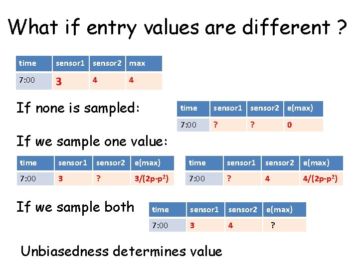
What if entry values are different ? time sensor 1 sensor 2 max 7: 00 3 4 4 If none is sampled: time sensor 1 sensor 2 e(max) 7: 00 ? ? 0 If we sample one value: time sensor 1 sensor 2 e(max) 7: 00 3 ? 3/(2 p-p 2) 7: 00 ? 4 4/(2 p-p 2) time sensor 1 sensor 2 e(max) 7: 00 3 4 If we sample both Unbiasedness determines value ?

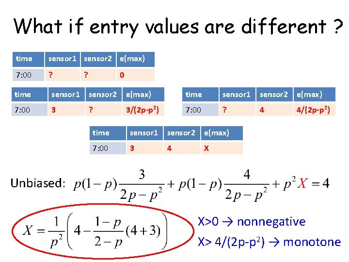
What if entry values are different ? time sensor 1 sensor 2 e(max) 7: 00 ? ? 0 time sensor 1 sensor 2 e(max) 7: 00 3 ? 3/(2 p-p 2) 7: 00 ? 4 4/(2 p-p 2) time sensor 1 sensor 2 e(max) 7: 00 3 4 X Unbiased: X>0 → nonnegative X> 4/(2 p-p 2) → monotone

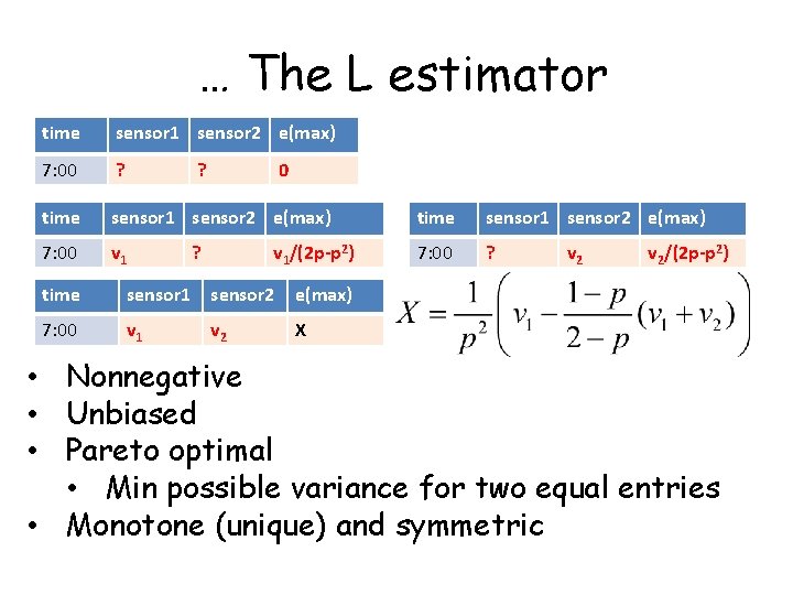
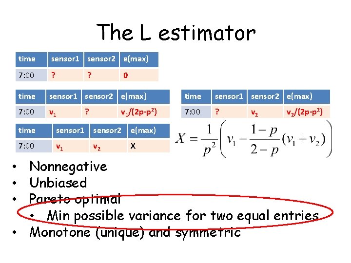
… The L estimator time sensor 1 sensor 2 e(max) 7: 00 ? time sensor 1 sensor 2 e(max) 7: 00 v 1 7: 00 ? ? 0 ? v 1/(2 p-p 2) time sensor 1 sensor 2 e(max) 7: 00 v 1 v 2 X v 2/(2 p-p 2) • Nonnegative • Unbiased • Pareto optimal • Min possible variance for two equal entries • Monotone (unique) and symmetric

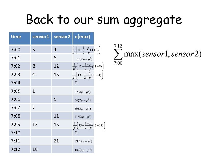
Back to our sum aggregate time sensor 1 sensor 2 e(max) 7: 00 3 7: 01 4 5 7: 02 8 12 7: 03 4 13 7: 04 7: 05 0 1 7: 06 7: 07 5 6 7: 08 7: 09 11 12 13 7: 10 0 7: 11 7: 12 21 10

The L estimator time sensor 1 sensor 2 e(max) 7: 00 ? time sensor 1 sensor 2 e(max) 7: 00 v 1 7: 00 ? ? 0 ? v 1/(2 p-p 2) time sensor 1 sensor 2 e(max) 7: 00 v 1 v 2 X v 2/(2 p-p 2) • Nonnegative • Unbiased • Pareto optimal • Min possible variance for two equal entries • Monotone (unique) and symmetric

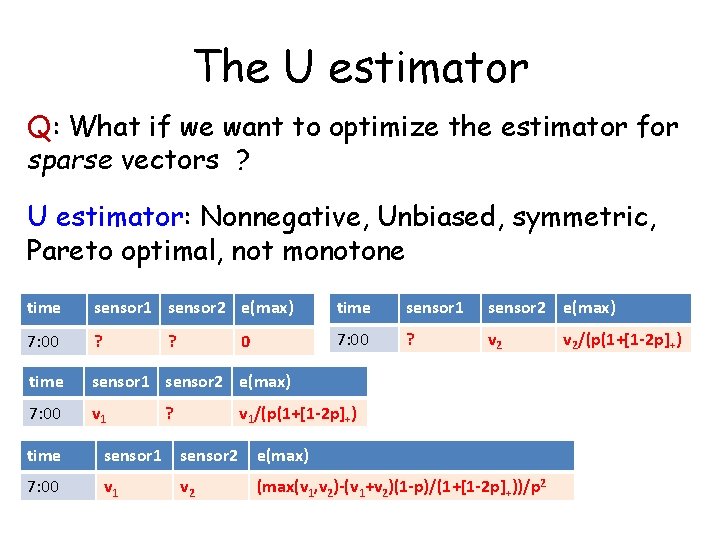
The U estimator Q: What if we want to optimize the estimator for sparse vectors ? U estimator: Nonnegative, Unbiased, symmetric, Pareto optimal, not monotone time sensor 1 sensor 2 e(max) 7: 00 ? v 2 time sensor 1 sensor 2 e(max) 7: 00 v 1 ? 0 ? v 1/(p(1+[1 -2 p]+) time sensor 1 sensor 2 e(max) 7: 00 v 1 v 2 (max(v 1, v 2)-(v 1+v 2)(1 -p)/(1+[1 -2 p]+))/p 2 v 2/(p(1+[1 -2 p]+)

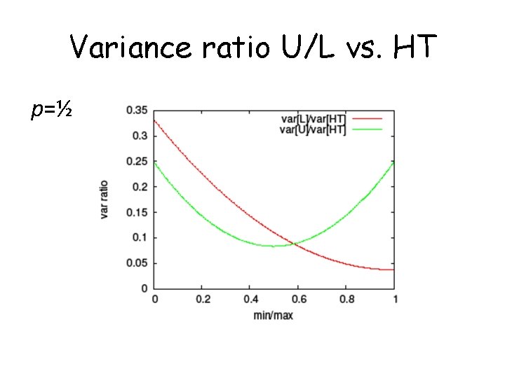
Variance ratio U/L vs. HT p=½

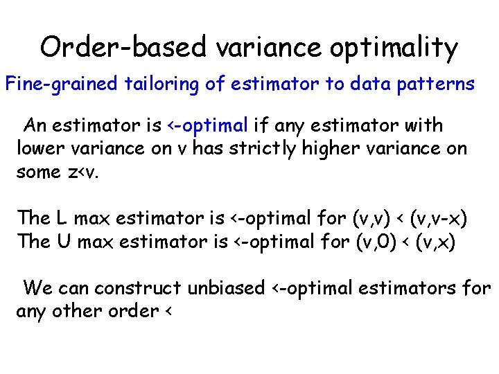
Order-based variance optimality Fine-grained tailoring of estimator to data patterns An estimator is ‹-optimal if any estimator with lower variance on v has strictly higher variance on some z<v. The L max estimator is <-optimal for (v, v) < (v, v-x) The U max estimator is <-optimal for (v, 0) < (v, x) We can construct unbiased <-optimal estimators for any other order <

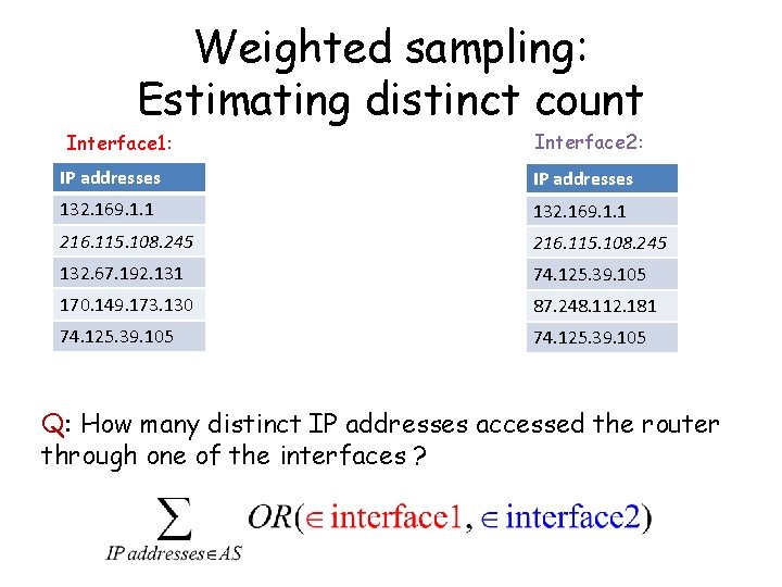
Weighted sampling: Estimating distinct count Interface 1: Interface 2: IP addresses 132. 169. 1. 1 216. 115. 108. 245 132. 67. 192. 131 74. 125. 39. 105 170. 149. 173. 130 87. 248. 112. 181 74. 125. 39. 105 Q: How many distinct IP addresses accessed the router through one of the interfaces ?

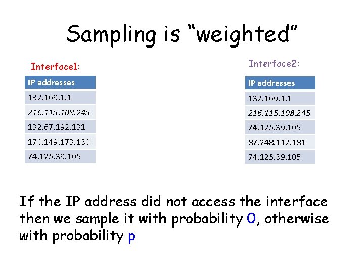
Sampling is “weighted” Interface 1: Interface 2: IP addresses 132. 169. 1. 1 216. 115. 108. 245 132. 67. 192. 131 74. 125. 39. 105 170. 149. 173. 130 87. 248. 112. 181 74. 125. 39. 105 If the IP address did not access the interface then we sample it with probability 0, otherwise with probability p

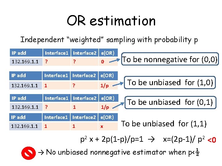
OR estimation Independent “weighted” sampling with probability p IP add Interface 1 Interface 2 e(OR) 132. 169. 1. 1 ? IP add Interface 1 Interface 2 e(OR) 132. 169. 1. 1 1 ? ? 1 1 0 1/p x To be nonnegative for (0, 0) To be unbiased for (1, 0) To be unbiased for (0, 1) To be unbiased for (1, 1) p 2 x + 2 p(1 -p)/p=1 → x=(2 p-1)/ p 2 <0 → No unbiased nonnegative estimator when p<½

Negative result (? ? ) Independent “weighted” sampling: There is no non-negative unbiased estimator for OR (related to M. Charikar, S. Chaudhuri, R. Motwani, and V. Narasayya (PODS 2000), negative results for distinct element counts) Same holds for other functions like the ℓ-th largest value (ℓ < d), and range (Lp difference) Known seeds: Same sampling scheme but we make random bits “public: ” can sometimes get information on values also when entry is not sampled (and get good estimators!)

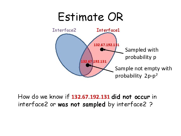
Estimate OR Interface 2 Interface 1 132. 67. 192. 131 Sampled with probability p Sample not empty with probability 2 p-p 2 How do we know if 132. 67. 192. 131 did not occur in interface 2 or was not sampled by interface 2 ?

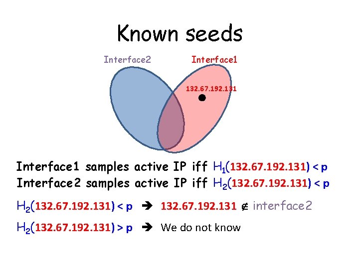
Known seeds Interface 2 Interface 1 132. 67. 192. 131 Interface 1 samples active IP iff H 1(132. 67. 192. 131) < p Interface 2 samples active IP iff H 2(132. 67. 192. 131) < p 132. 67. 192. 131 interface 2 H 2(132. 67. 192. 131) > p We do not know

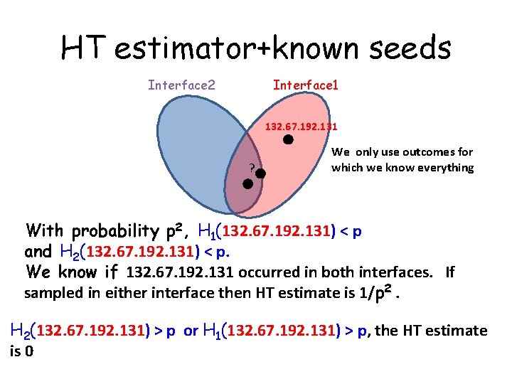
HT estimator+known seeds Interface 2 Interface 1 132. 67. 192. 131 ? We only use outcomes for which we know everything With probability p 2, H 1(132. 67. 192. 131) < p and H 2(132. 67. 192. 131) < p. We know if 132. 67. 192. 131 occurred in both interfaces. If sampled in either interface then HT estimate is 1/p 2. H 2(132. 67. 192. 131) > p or H 1(132. 67. 192. 131) > p, the HT estimate is 0

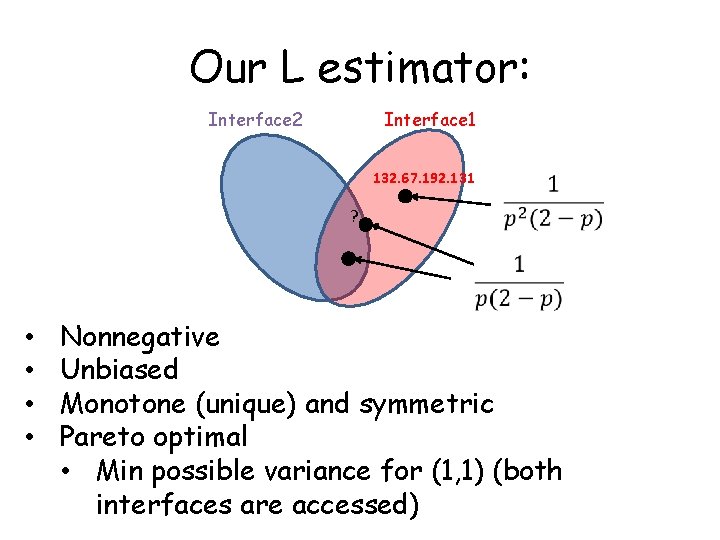
Our L estimator: Interface 2 Interface 1 132. 67. 192. 131 ? • • Nonnegative Unbiased Monotone (unique) and symmetric Pareto optimal • Min possible variance for (1, 1) (both interfaces are accessed)

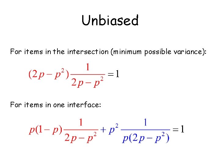
Unbiased For items in the intersection (minimum possible variance): For items in one interface:

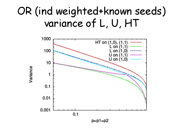
OR (ind weighted+known seeds) variance of L, U, HT

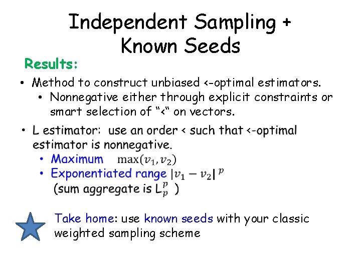
Independent Sampling + Known Seeds Results: • Method to construct unbiased <-optimal estimators. • Nonnegative either through explicit constraints or smart selection of “<“ on vectors. Take home: use known seeds with your classic weighted sampling scheme

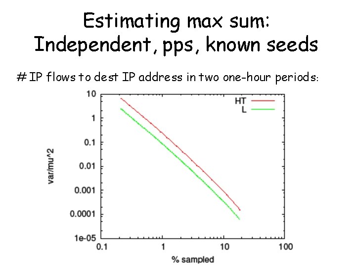
Estimating max sum: Independent, pps, known seeds # IP flows to dest IP address in two one-hour periods :

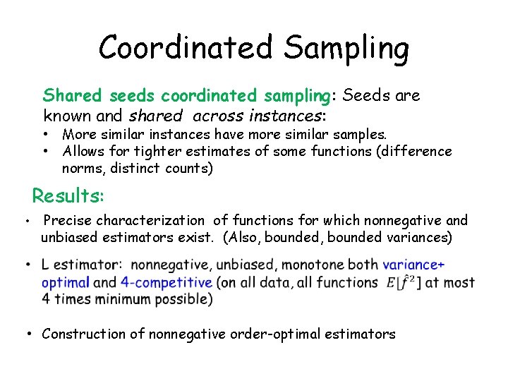
Coordinated Sampling Shared seeds coordinated sampling: Seeds are known and shared across instances: • More similar instances have more similar samples. • Allows for tighter estimates of some functions (difference norms, distinct counts) Results: • Precise characterization of functions for which nonnegative and unbiased estimators exist. (Also, bounded variances) • Construction of nonnegative order-optimal estimators

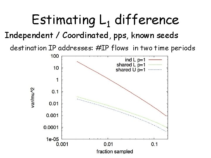
Estimating L 1 difference Independent / Coordinated, pps, known seeds destination IP addresses: #IP flows in two time periods

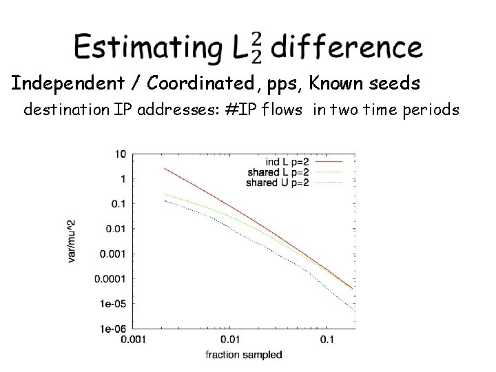
Independent / Coordinated, pps, Known seeds destination IP addresses: #IP flows in two time periods

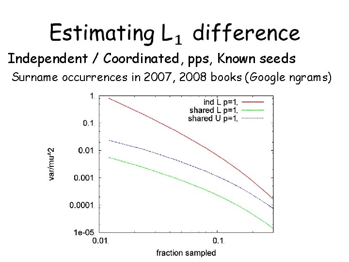
Independent / Coordinated, pps, Known seeds Surname occurrences in 2007, 2008 books (Google ngrams)

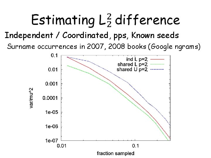
Independent / Coordinated, pps, Known seeds Surname occurrences in 2007, 2008 books (Google ngrams)

Conclusion • We present estimators for sum aggregates over samples: unbiased, nonnegative, variance optimal – Tailoring estimator to data (<-optimality) – Classic sampling schemes: independent/coordinated weighted/weight-oblivious Open/future: independent sampling (weighted+known seeds): precise characterization, derivation for >2 instances