Geomorphometry I Terrain modeling Geospatial Analysis and Modeling

Geomorphometry I: Terrain modeling Geospatial Analysis and Modeling: Lecture notes Helena Mitasova, NCSU MEAS Geospatial Analysis and Modeling - NCSU MEAS – Helena Mitasova

Outline • • Definitions 3 D mapping technologies mathematical and digital terrain models point clouds, multiple return data triangular irregular networks regular grid (raster) isolines and meshes point cloud analysis and binning Geospatial Analysis and Modeling - NCSU MEAS – Helena Mitasova

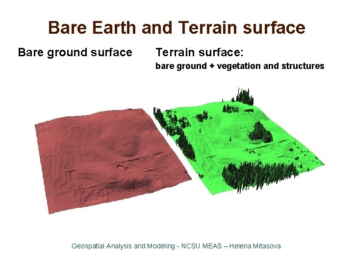
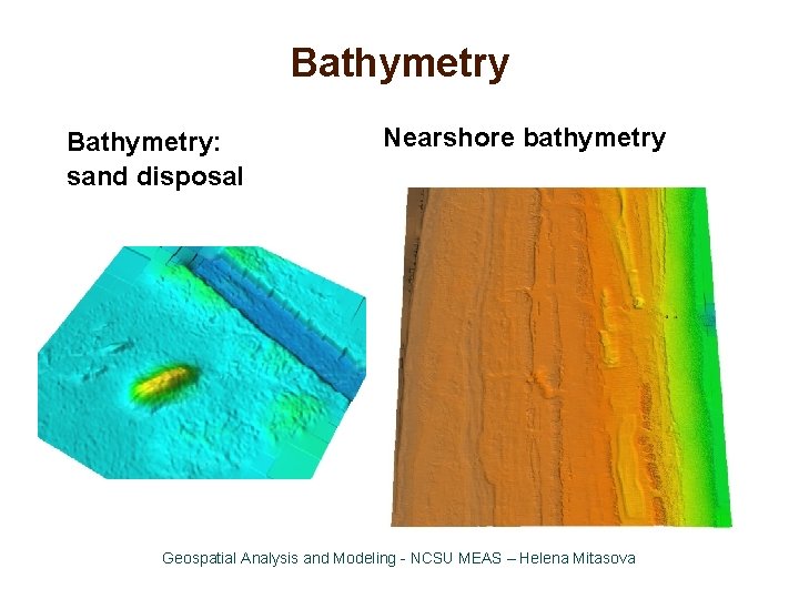
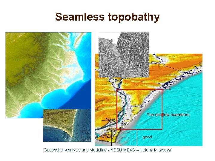
Definitions • Land (bare earth) surface: interface between solid Earth and atmosphere/anthroposphere/biosphere • Terrain surface : interface between Earth with water, vegetation, structures and atmosphere • Bathymetry: interface between solid Earth surface and hydrosphere (bottom surface of lakes, rivers and ocean) • Seamless topobathy: continuous solid earth surface Geospatial Analysis and Modeling - NCSU MEAS – Helena Mitasova

Bare Earth and Terrain surface Bare ground surface Terrain surface: bare ground + vegetation and structures Geospatial Analysis and Modeling - NCSU MEAS – Helena Mitasova

Bathymetry: sand disposal Nearshore bathymetry Geospatial Analysis and Modeling - NCSU MEAS – Helena Mitasova

Seamless topobathy Geospatial Analysis and Modeling - NCSU MEAS – Helena Mitasova

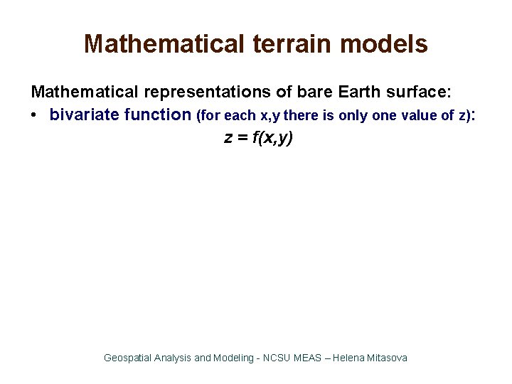
Mathematical terrain models Mathematical representations of bare Earth surface: • bivariate function (for each x, y there is only one value of z): z = f(x, y) Geospatial Analysis and Modeling - NCSU MEAS – Helena Mitasova

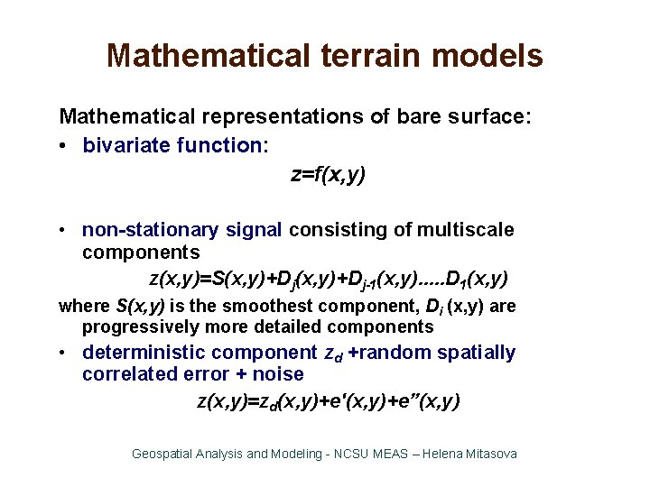
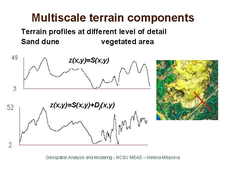
Mathematical terrain models Mathematical representations of bare surface: • bivariate function: z=f(x, y) • non-stationary signal consisting of multiscale components z(x, y)=S(x, y)+Dj-1(x, y). . . D 1(x, y) where S(x, y) is the smoothest component, Di (x, y) are progressively more detailed components • deterministic component zd +random spatially correlated error + noise z(x, y)=zd(x, y)+e'(x, y)+e”(x, y) Geospatial Analysis and Modeling - NCSU MEAS – Helena Mitasova

Multiscale terrain components Terrain profiles at different level of detail Sand dune vegetated area z(x, y)=S(x, y)+Dj(x, y) Geospatial Analysis and Modeling - NCSU MEAS – Helena Mitasova

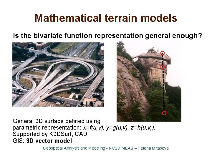
Mathematical terrain models Is the bivariate function representation general enough? General 3 D surface defined using parametric representation: x=f(u, v), y=g(u, v), z=h(u, v, ), Supported by K 3 DSurf, CAD GIS: 3 D vector model Geospatial Analysis and Modeling - NCSU MEAS – Helena Mitasova

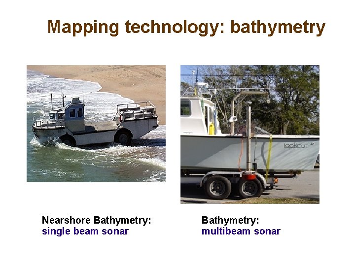
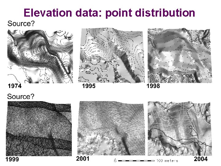
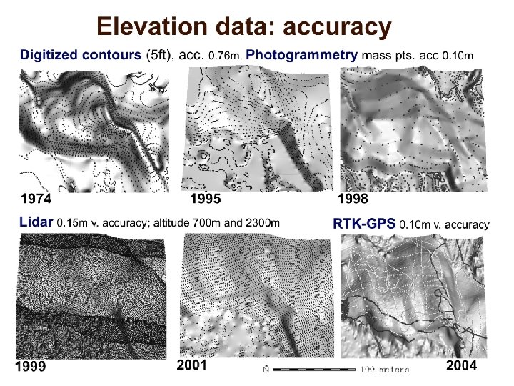
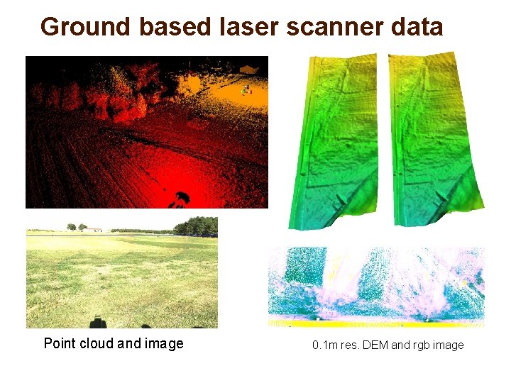
Terrain mapping technologies Continuous surface measured at discrete points • Human selected points (GPS, total station, photogrammetry) • Automated point sampling (lidar, RTK GPS, sonar) Land terrain mapping • • Stereophotogrammetry: mass points and breaklines IFSARE: raster, Lidar: point cloud On-ground 3 d laser scanner: point cloud RTK GPS: point profiles Bathymetry mapping single and multiple beam sonar Geospatial Analysis and Modeling - NCSU MEAS – Helena Mitasova

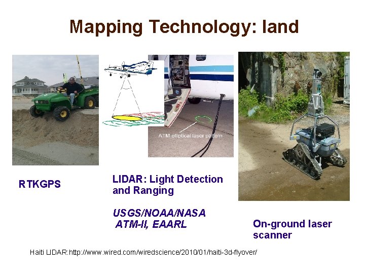
Mapping Technology: land RTKGPS LIDAR: Light Detection and Ranging USGS/NOAA/NASA ATM-II, EAARL On-ground laser scanner Haiti LIDAR: http: //www. wired. com/wiredscience/2010/01/haiti-3 d-flyover/

Mapping technology: bathymetry Nearshore Bathymetry: single beam sonar Bathymetry: multibeam sonar

Elevation data: point distribution

Elevation data: accuracy

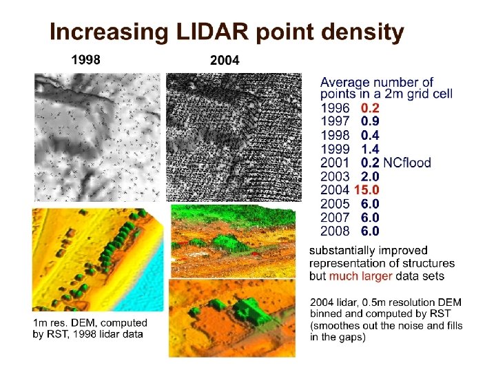
substantially improved representation of structures but much larger data sets 1 m res. DEM, computed by RST, 1998 lidar data 2004 lidar, 0. 5 m resolution DEM binned and computed by RST (smoothes out the noise and fills in the gaps)

Ground based laser scanner data Point cloud and image 0. 1 m res. DEM and rgb image

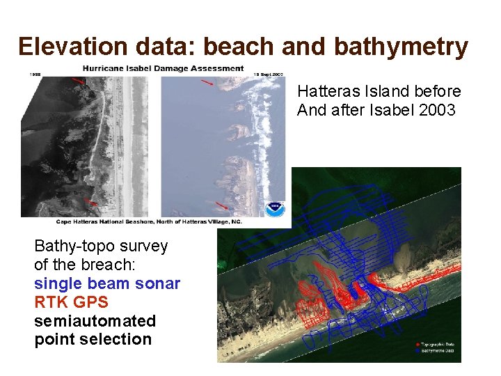
Elevation data: beach and bathymetry Hatteras Island before And after Isabel 2003 Bathy-topo survey of the breach: single beam sonar RTK GPS semiautomated point selection

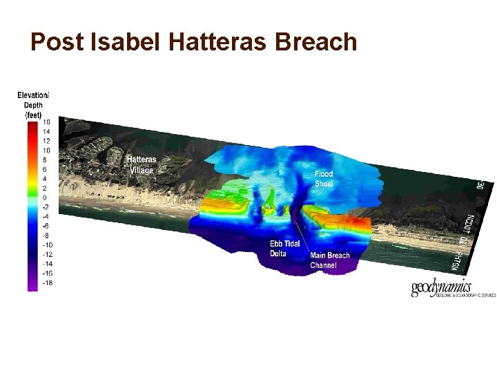
Post Isabel Hatteras Breach

Digital terrain representations • Point clouds – measured data • TIN – Triangular Irregular Network • Regular grid (raster) • Contours - elevation isolines • Mesh Geospatial Analysis and Modeling - NCSU MEAS – Helena Mitasova

Point clouds • Set of (x, y, z, r, i, . . . ) measured points reflected from Earth surface or objects on or above it, where x, y, z are georeferenced coordinates, r is the return number and i is intensity, r: g: b may be also measured • Provided in – ASCII (x, y, z, . . . ) format – binary LAS format (header, record info, x, y, z, i, scan dir, edge of flight line, classification, etc. ), industry lidar data exchange format Geospatial Analysis and Modeling - NCSU MEAS – Helena Mitasova

Point clouds Processing: – – filtering outliers (birds etc. ) bare earth point extraction canopy extraction structures and power lines extraction Public data sources (http in Summary slide): CLICK: raw point clouds usually in LAS format LDART: costal point clouds with on-fly binning NC Floodplain Mapping: bare Earth: points, 20 ft DEM and 50 ft DEM with carved channels Geospatial Analysis and Modeling - NCSU MEAS – Helena Mitasova

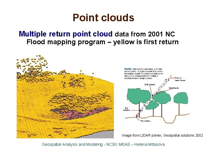
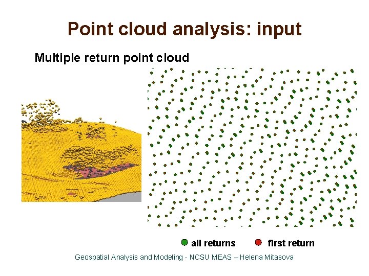
Point clouds Multiple return point cloud data from 2001 NC Flood mapping program – yellow is first return Image from LIDAR primer, Geospatial solutions 2002 Geospatial Analysis and Modeling - NCSU MEAS – Helena Mitasova

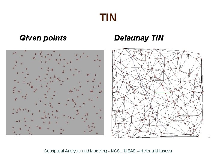
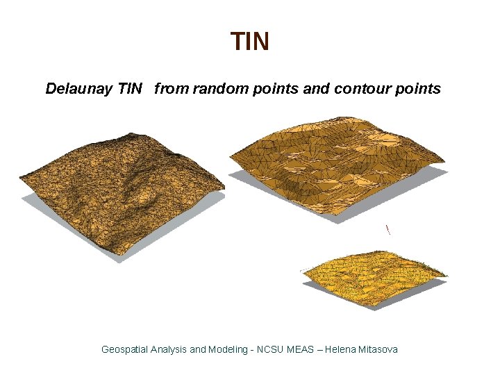
TIN • Triangular Irregular Network: constructed from the measured points by triangulation (before computer age this technique was used for manual interpolation of contours from surveyed points) • Delaunay Triangulation: maximizes the smallest angle of the triangles to avoid skinny triangles • Constrained Delaunay Triangulation – includes predefined edges that cannot be flipped • TIN is a vector data model representation, that usually preserves the original data points Geospatial Analysis and Modeling - NCSU MEAS – Helena Mitasova

TIN Given points Delaunay TIN Geospatial Analysis and Modeling - NCSU MEAS – Helena Mitasova

TIN Delaunay TIN from random points and contour points Geospatial Analysis and Modeling - NCSU MEAS – Helena Mitasova

TIN properties • requires pre-defined breaklines for man-made features, valleys, faults, etc. • density of TIN is adjusted to surface complexity • additional points may need to be interpolated to create smooth surface When to use TIN: • engineering applications, • manual modification of model is desired(design), • complex faults need to be represented, • multiscale representation for visualization Geospatial Analysis and Modeling - NCSU MEAS – Helena Mitasova

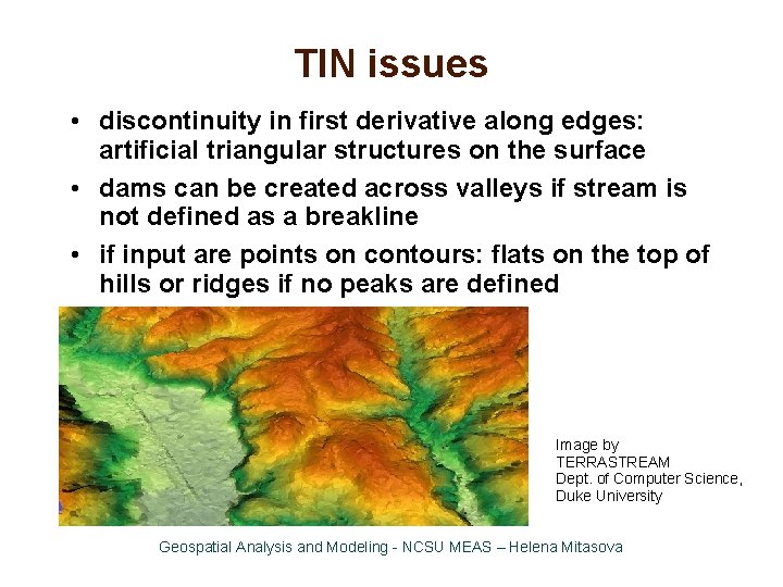
TIN issues • discontinuity in first derivative along edges: artificial triangular structures on the surface • dams can be created across valleys if stream is not defined as a breakline • if input are points on contours: flats on the top of hills or ridges if no peaks are defined Image by TERRASTREAM Dept. of Computer Science, Duke University Geospatial Analysis and Modeling - NCSU MEAS – Helena Mitasova

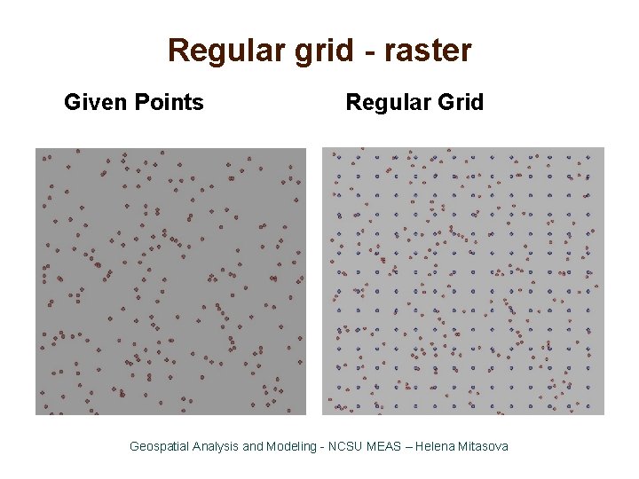
Regular grid - raster Two interpretations: • elevation assigned to a grid point – center of the grid cell • elevation assigned to the pixel area Derived from measured points by gridding: • at least one point for each grid cell – binning, • if some grid cells do not include points – spatial interpolation or approximation Geospatial Analysis and Modeling - NCSU MEAS – Helena Mitasova

Regular grid - raster Given Points Regular Grid Geospatial Analysis and Modeling - NCSU MEAS – Helena Mitasova

Regular grid: properties • simple data structure and algorithms • easy to combine with imagery • uniform resolution - potential for undersampling and oversampling • representation of faults and sharp breaklines requires very high resolution Geospatial Analysis and Modeling - NCSU MEAS – Helena Mitasova

Regular grid -public data Most available elevation data are distributed as raster data: • USGS Seamless Data Distribution – NED 1/9 (3 m), 1/3 (10 m), 1 arc/sec (30 m), • SRTM-V 4: USA 30 m, World 90 m • GDEM 15 -30 m: global, relative height, derived from ASTER satellite stereo bands • NCFlood mapping web site: 20 ft and 50 ft DEM • CRM for bathymetry: 90 m • Seamless Topobathy: Tsunami data and RENCI NC data 10 m Geospatial Analysis and Modeling - NCSU MEAS – Helena Mitasova

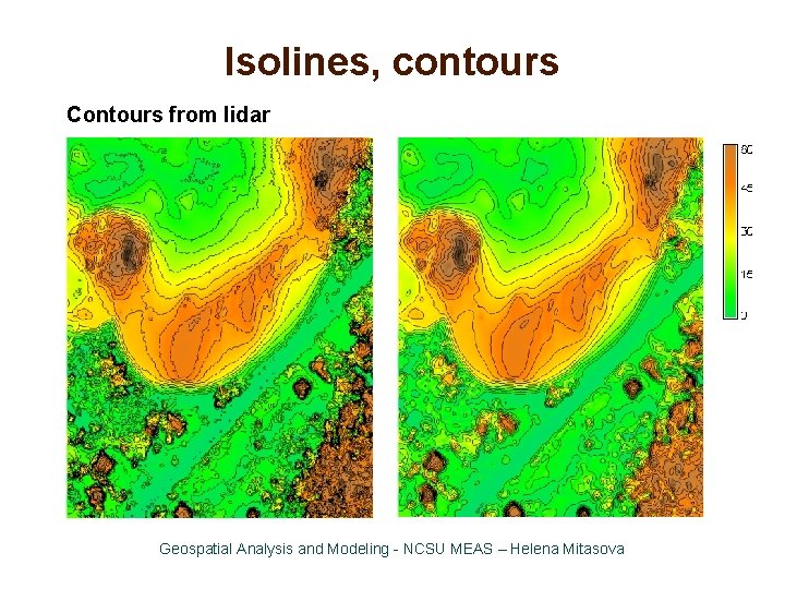
Isolines, contours • traditional approach for representation of elevation, drawn by hand from measured mass points by interpolating along triangle edges • automated procedures: from TIN or grid, • not very suitable for highly detailed, noisy data such as lidar • needed when the surface has simple geometry • selecting contour interval: depends on slope and resolution Geospatial Analysis and Modeling - NCSU MEAS – Helena Mitasova

Isolines, contours Contours from lidar Geospatial Analysis and Modeling - NCSU MEAS – Helena Mitasova

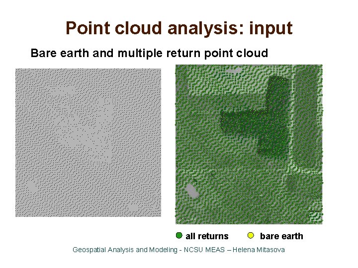
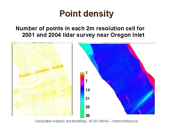
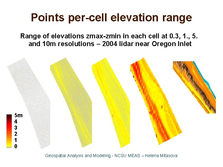
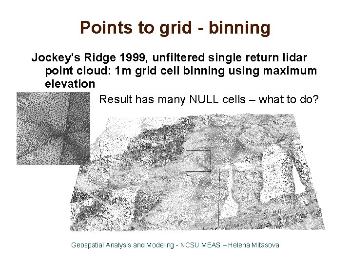
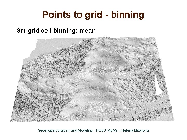
Point cloud analysis: binning Binning: fast method for analyzing point clouds and generating DEMs using per-cell processing: • at least one point for each grid cell • analysis: number of points per cell, range, stddv • Methods for DEM: mean, min, max, nearest • sufficient for many applications • no need to import the points, on-fly raster generation • may be noisy, include no-data spots Geospatial Analysis and Modeling - NCSU MEAS – Helena Mitasova

Point cloud analysis: input Multiple return point cloud all returns first return Geospatial Analysis and Modeling - NCSU MEAS – Helena Mitasova

Point cloud analysis: input Bare earth and multiple return point cloud all returns bare earth Geospatial Analysis and Modeling - NCSU MEAS – Helena Mitasova

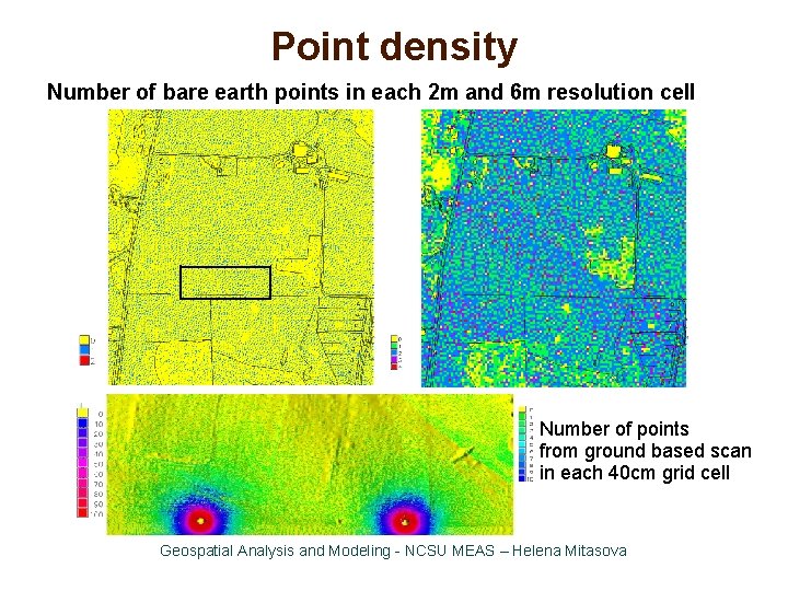
Point density Number of bare earth points in each 2 m and 6 m resolution cell Number of points from ground based scan in each 40 cm grid cell Geospatial Analysis and Modeling - NCSU MEAS – Helena Mitasova

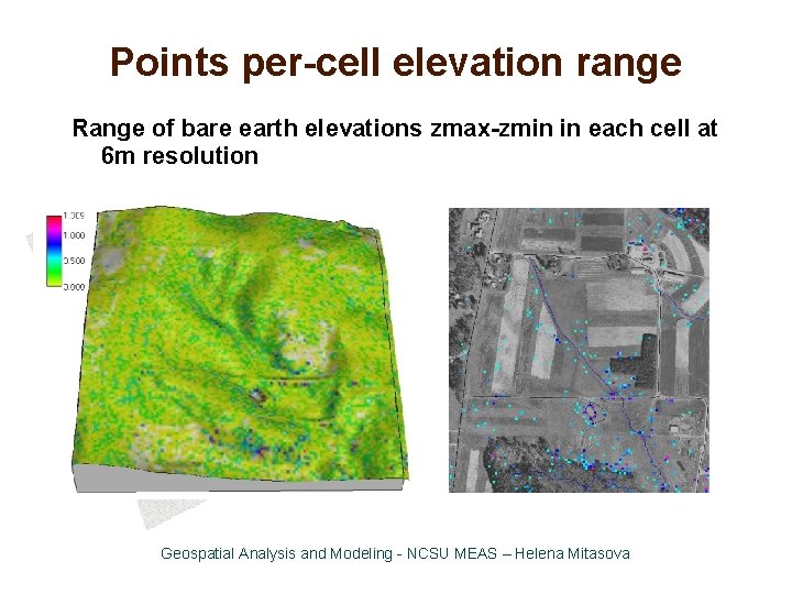
Points per-cell elevation range Range of bare earth elevations zmax-zmin in each cell at 6 m resolution Geospatial Analysis and Modeling - NCSU MEAS – Helena Mitasova

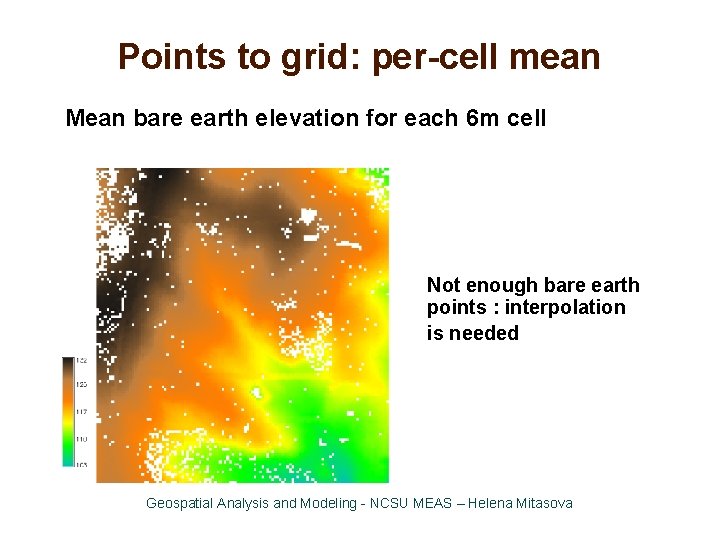
Points to grid: per-cell mean Mean bare earth elevation for each 6 m cell Not enough bare earth points : interpolation is needed Geospatial Analysis and Modeling - NCSU MEAS – Helena Mitasova

Point density Number of points in each 2 m resolution cell for 2001 and 2004 lidar survey near Oregon Inlet 1 7 14 21 28 35 Geospatial Analysis and Modeling - NCSU MEAS – Helena Mitasova

Points per-cell elevation range Range of elevations zmax-zmin in each cell at 0. 3, 1. , 5. and 10 m resolutions – 2004 lidar near Oregon Inlet 5 m 4 3 2 1 0 Geospatial Analysis and Modeling - NCSU MEAS – Helena Mitasova

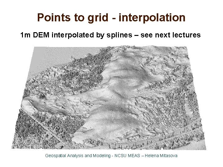
Points to grid - binning Jockey's Ridge 1999, unfiltered single return lidar point cloud: 1 m grid cell binning using maximum elevation Result has many NULL cells – what to do? Geospatial Analysis and Modeling - NCSU MEAS – Helena Mitasova

Points to grid - binning 3 m grid cell binning: mean Geospatial Analysis and Modeling - NCSU MEAS – Helena Mitasova

Points to grid - interpolation 1 m DEM interpolated by splines – see next lectures Geospatial Analysis and Modeling - NCSU MEAS – Helena Mitasova

Summary and references • Mathematical and digital terrain representation – Hegl CH. 2 Chang Ch. X, Neteler Ch. 5, 6 • Point clouds and TIN – Hegl, Chang Ch. X, Neteler Ch. 6. • Regular grids – Hegl, Neteler Ch. 7, others • Isolines and meshes – Hegl, Neteler Ch 5 Links to elevation data distribution sites see http: //skagit. meas. ncsu. edu/~helena/classwork/hon 297 webgis. html LIDAR: http: //www. forestry. gov. uk/forestry/INFD-6 RVC 9 J http: //www. geospatial-solutions. com/geospatialsolutions/article. Detail. jsp? id=10275 Geospatial Analysis and Modeling - NCSU MEAS – Helena Mitasova