Food and Agricultural Policy Stylized Facts and Hypothesis

Food and Agricultural Policy: Stylized Facts and Hypothesis Tests Will Masters Andres Garcia wmasters@purdue. edu www. agecon. purdue. edu/staff/masters andres@purdue. edu www. andresgarcia. net 28 May 2008

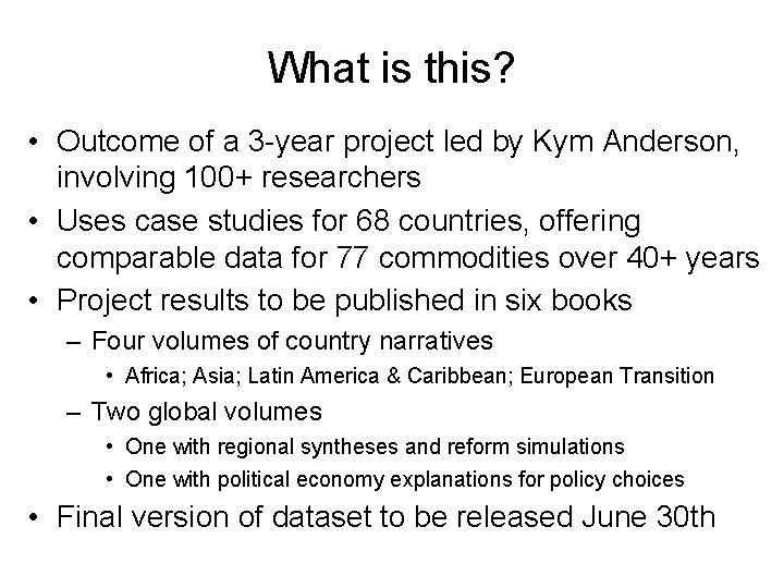
What is this? • Outcome of a 3 -year project led by Kym Anderson, involving 100+ researchers • Uses case studies for 68 countries, offering comparable data for 77 commodities over 40+ years • Project results to be published in six books – Four volumes of country narratives • Africa; Asia; Latin America & Caribbean; European Transition – Two global volumes • One with regional syntheses and reform simulations • One with political economy explanations for policy choices • Final version of dataset to be released June 30 th

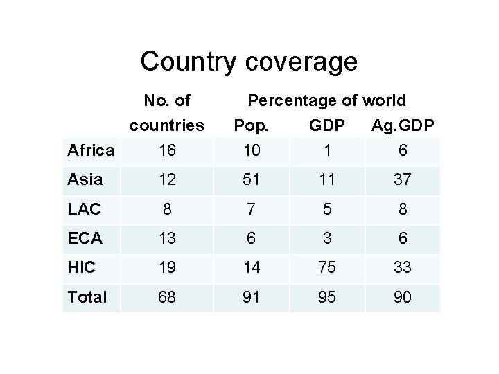
Country coverage No. of countries Africa 16 Percentage of world Pop. GDP Ag. GDP 10 1 6 Asia 12 51 11 37 LAC 8 7 5 8 ECA 13 6 HIC 19 14 75 33 Total 68 91 95 90

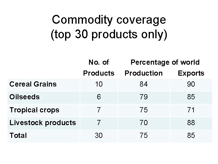
Commodity coverage (top 30 products only) Cereal Grains No. of Products 10 Percentage of world Production Exports 84 90 Oilseeds 6 79 85 Tropical crops 7 75 71 Livestock products 7 70 88 Total 30 75 85

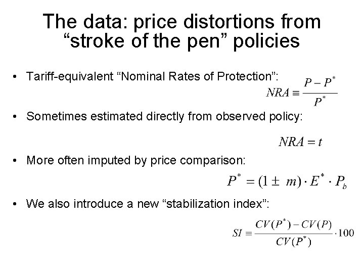
The data: price distortions from “stroke of the pen” policies • Tariff-equivalent “Nominal Rates of Protection”: • Sometimes estimated directly from observed policy: • More often imputed by price comparison: • We also introduce a new “stabilization index”:

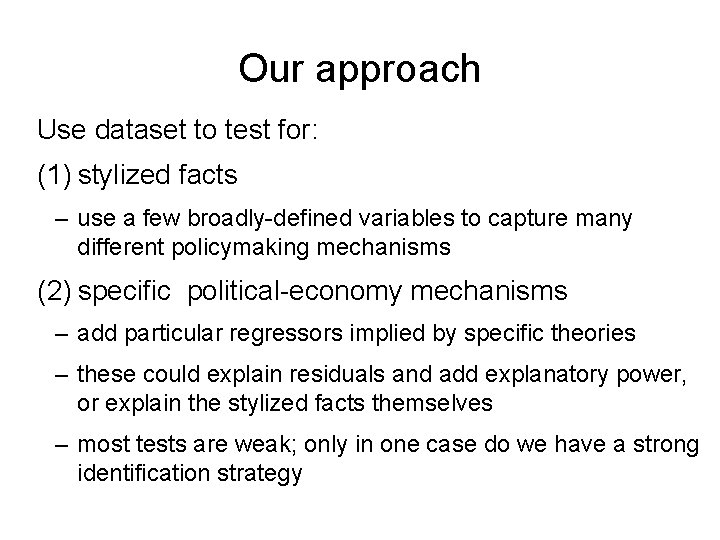
Our approach Use dataset to test for: (1) stylized facts – use a few broadly-defined variables to capture many different policymaking mechanisms (2) specific political-economy mechanisms – add particular regressors implied by specific theories – these could explain residuals and add explanatory power, or explain the stylized facts themselves – most tests are weak; only in one case do we have a strong identification strategy

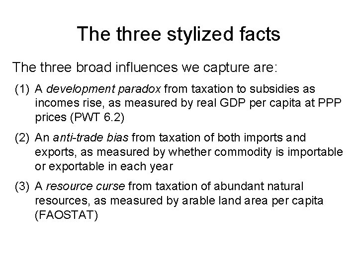
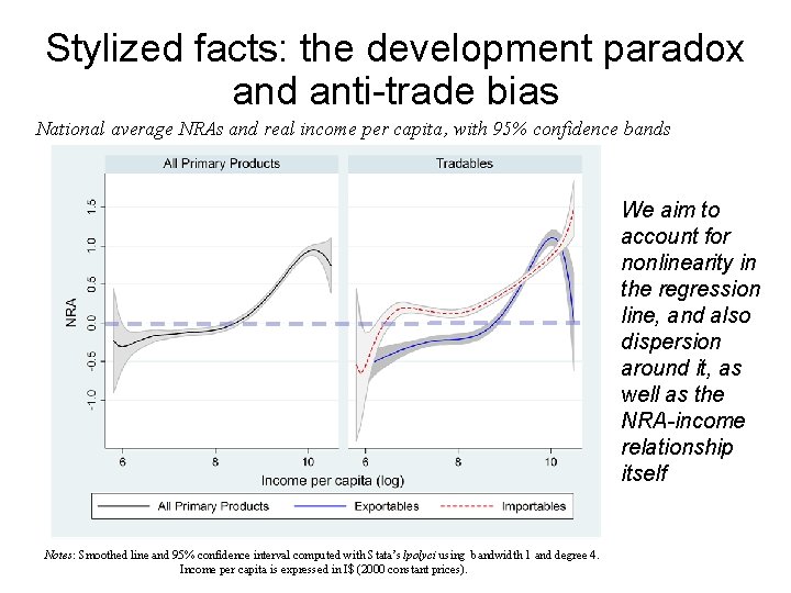
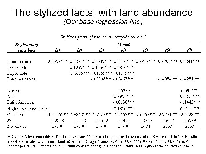
The three stylized facts The three broad influences we capture are: (1) A development paradox from taxation to subsidies as incomes rise, as measured by real GDP per capita at PPP prices (PWT 6. 2) (2) An anti-trade bias from taxation of both imports and exports, as measured by whether commodity is importable or exportable in each year (3) A resource curse from taxation of abundant natural resources, as measured by arable land area per capita (FAOSTAT)

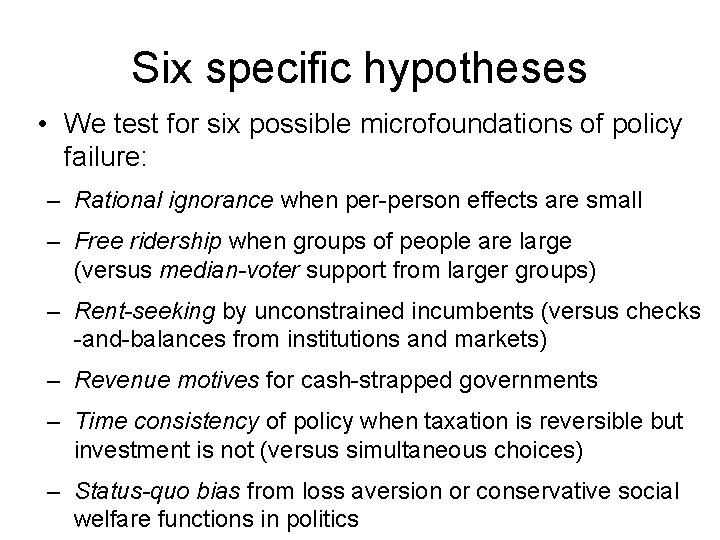
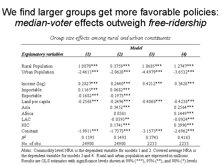
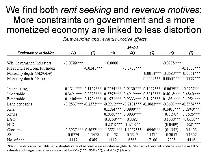
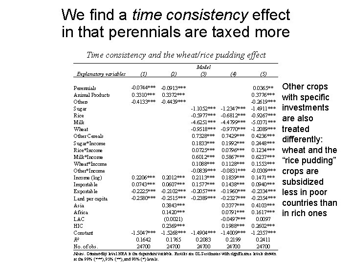
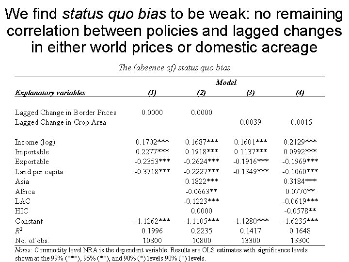
Six specific hypotheses • We test for six possible microfoundations of policy failure: – Rational ignorance when per-person effects are small – Free ridership when groups of people are large (versus median-voter support from larger groups) – Rent-seeking by unconstrained incumbents (versus checks -and-balances from institutions and markets) – Revenue motives for cash-strapped governments – Time consistency of policy when taxation is reversible but investment is not (versus simultaneous choices) – Status-quo bias from loss aversion or conservative social welfare functions in politics

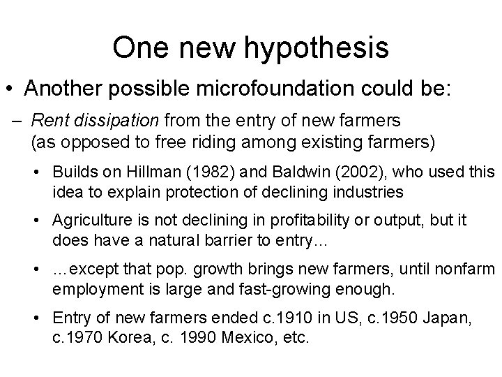
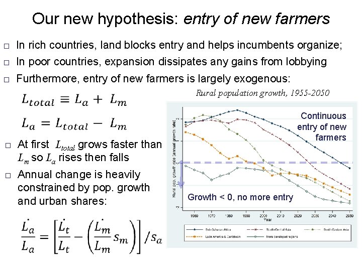
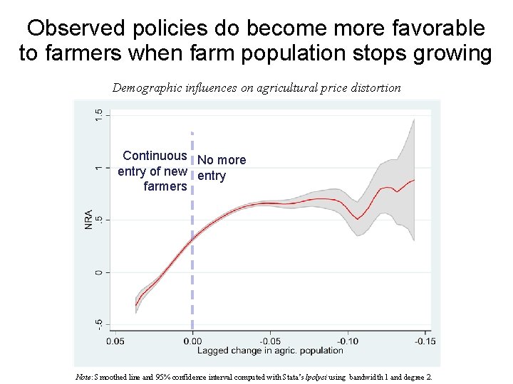
One new hypothesis • Another possible microfoundation could be: – Rent dissipation from the entry of new farmers (as opposed to free riding among existing farmers) • Builds on Hillman (1982) and Baldwin (2002), who used this idea to explain protection of declining industries • Agriculture is not declining in profitability or output, but it does have a natural barrier to entry… • …except that pop. growth brings new farmers, until nonfarm employment is large and fast-growing enough. • Entry of new farmers ended c. 1910 in US, c. 1950 Japan, c. 1970 Korea, c. 1990 Mexico, etc.

Stylized facts: the development paradox and anti-trade bias National average NRAs and real income per capita, with 95% confidence bands We aim to account for nonlinearity in the regression line, and also dispersion around it, as well as the NRA-income relationship itself Notes: Smoothed line and 95% confidence interval computed with Stata’s lpolyci using bandwidth 1 and degree 4. Income per capita is expressed in I$ (2000 constant prices).

The stylized facts, with land abundance (Our base regression line) Stylized facts of the commodity-level NRA Explanatory variables Income (log) Importable Exportable Land per capita (1) (2) (3) Model (4) (5) (6) (7) 0. 2553*** 0. 2277*** 0. 2549*** 0. 2186*** 0. 3383*** 0. 3700*** 0. 2841*** 0. 1939*** 0. 1136*** 0. 0884*** -0. 1685*** -0. 1859*** -0. 1875*** -0. 2508*** -0. 2467*** -0. 4084*** -0. 4281*** Africa 0. 0289 0. 0956** Asia 0. 2955*** 0. 2253*** Latin America -0. 0638*** -0. 1442*** High income countries 0. 1856*** 0. 4152*** Constant -1. 8905*** -1. 6868*** -1. 7727*** -1. 5653*** -2. 6407*** -2. 7731*** -2. 2228*** R 2 0. 0848 0. 1152 0. 1349 0. 1456 0. 2705 0. 3467 0. 3989 No. of obs. 27600 24900 2484 2233 Notes: NRA by commodity is the dependent variable for models 1 -4 is and covered total NRA for models 5 -7. Results are OLS estimates with robust standard errors and significance levels at 99% (***), 95% (**), and 90% (*) levels. Income per capita is expressed in I$ (2000 constant prices). Europe and Central Asia region is the omitted continent.

The stylized facts are (slightly) different within regions National average NRAs and real income per capita, by region Notes: Smoothed line and 95% confidence interval computed with Stata’s lpolyci using bandwidth 1 and degree 4. Income per capita is expressed in I$ (2000 constant prices).

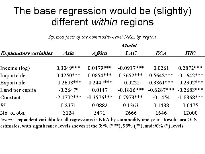
The base regression would be (slightly) different within regions Stylized facts of the commodity-level NRA, by region Explanatory variables Income (log) Importable Exportable Land per capita Constant R 2 No. of obs. Asia Africa Model LAC ECA HIC 0. 3049*** 0. 0479*** -0. 0917*** 0. 0261 0. 2872*** 0. 4250*** 0. 0854*** 0. 3652*** 0. 5642*** -0. 1642*** -0. 2603*** -0. 2447*** -0. 0225 0. 3361*** -0. 2902*** -0. 2647* 0. 0147 -0. 1836*** -0. 6287*** -0. 2683*** -2. 1702*** -0. 3576*** 0. 7973*** -0. 1454 -1. 8368*** 0. 2371 0. 0882 0. 1363 0. 1438 0. 0475 3124 5471 2666 1646 12000 Notes: Dependent variable for all regressions is NRA by commodity and year. Results are OLS estimates, with significance levels shown at the 99% (***), 95% (**), and 90% (*) levels.

There is also (some) time-series variation we can exploit National average NRA over time, by region Note: Smoothed line and 95% confidence interval computed with Stata’s lpolyci using bandwidth 1 and degree 2.

Can we explain trend changes in the stylized facts, e. g. less anti-trade bias? National average NRA over time, by region and trade direction Note: Smoothed line and 95% confidence interval computed with Stata’s lpolyci using bandwidth 1 and degree 2.

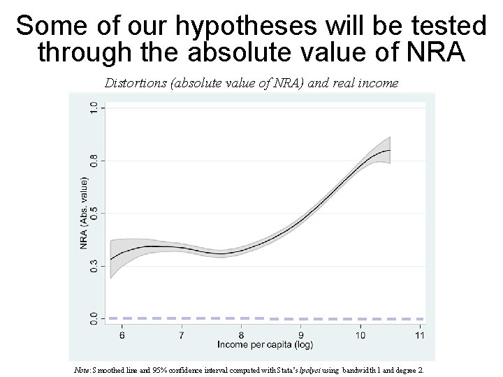
Some of our hypotheses will be tested through the absolute value of NRA Distortions (absolute value of NRA) and real income Note: Smoothed line and 95% confidence interval computed with Stata’s lpolyci using bandwidth 1 and degree 2.

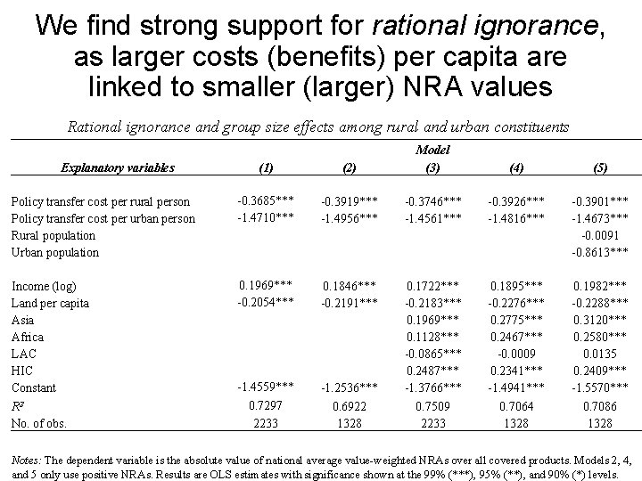
We find strong support for rational ignorance, as larger costs (benefits) per capita are linked to smaller (larger) NRA values Rational ignorance and group size effects among rural and urban constituents (1) (2) Model (3) Policy transfer cost per rural person Policy transfer cost per urban person Rural population Urban population -0. 3685*** -1. 4710*** -0. 3919*** -1. 4956*** -0. 3746*** -1. 4561*** -0. 3926*** -1. 4816*** -0. 3901*** -1. 4673*** -0. 0091 -0. 8613*** Income (log) Land per capita Asia Africa LAC HIC Constant 0. 1969*** -0. 2054*** 0. 1846*** -0. 2191*** -1. 4559*** 0. 7297 2233 -1. 2536*** 0. 1722*** -0. 2183*** 0. 1969*** 0. 1128*** -0. 0865*** 0. 2487*** -1. 3766*** 0. 1895*** -0. 2276*** 0. 2775*** 0. 2467*** -0. 0009 0. 2341*** -1. 4941*** 0. 1982*** -0. 2288*** 0. 3120*** 0. 2580*** 0. 0135 0. 2409*** -1. 5570*** 0. 6922 1328 0. 7509 2233 0. 7064 1328 0. 7086 1328 Explanatory variables R 2 No. of obs. (4) (5) Notes: The dependent variable is the absolute value of national average value-weighted NRAs over all covered products. Models 2, 4, and 5 only use positive NRAs. Results are OLS estimates with significance shown at the 99% (***), 95% (**), and 90% (*) levels.

We find larger groups get more favorable policies: median-voter effects outweigh free-ridership Group size effects among rural and urban constituents Model Explanatory variables (1) (2) (3) (4) Rural Population Urban Population 1. 0870*** -2. 4613*** 0. 3759*** -2. 0620*** 1. 8685*** -4. 4979*** 1. 2747*** -3. 6532*** Income (log) Importable Exportable Land per capita Asia Africa LAC HIC Constant R 2 No. of obs. 0. 2827*** 0. 1165*** -0. 1682*** -0. 2568*** 0. 2440*** 0. 0682*** -0. 1973*** -0. 2496*** 0. 3452*** 0. 0361 -0. 0393** 0. 1741*** -1. 7373*** 0. 1493 24900 0. 4212*** 0. 3428*** -0. 4060*** -0. 4238*** 0. 2564*** 0. 1449*** -0. 0924*** 0. 3990*** -2. 6962*** 0. 4163 2233 -1. 9911*** 0. 1395 24900 -3. 1573*** 0. 3743 2233 Notes: Commodity level NRA is the dependent variable for models 1 and 2. Covered average NRA is the dependent variable for models 3 and 4. Rural and urban population are expressed in millions. Results are OLS estimates with significance levels shown at 99% (***), 95% (**), and 90% (*) levels.

We find both rent seeking and revenue motives: More constraints on government and a more monetized economy are linked to less distortion Rent-seeking and revenue-motive effects Explanatory variables (1) (2) (3) Model (4) 0. 0000 (5) (6) (7) WB Governance Indicators Freedom Hse Econ. Fr. Index Monetary depth (M 2/GDP) Monetary depth * Income -0. 0799*** Income (log) Importable Exportable Land per capita Asia Africa LAC HIC Constant R 2 No. of obs. 0. 1311*** 0. 1157*** 0. 2254*** 0. 2130*** 0. 1697*** 0. 0629** 0. 0757** 0. 3421*** 0. 3898*** 0. 3797*** 0. 4212*** 0. 5018*** 0. 4840*** 0. 1406*** 0. 1796*** 0. 1971*** 0. 2333*** 0. 1470*** 0. 1851*** 0. 1954*** -0. 2837*** -0. 2373*** -0. 2212*** -0. 2101*** -0. 3083*** -0. 3607*** -0. 3554*** 0. 3384*** 0. 3900*** 0. 3401*** 0. 2840*** 0. 3060*** 0. 3033*** 0. 1150* 0. 1626*** -0. 0750*** 0. 0087 -0. 1530*** -0. 0630** -0. 2318*** 0. 0748** (0. 0409) 0. 3821*** -0. 8937*** -0. 5637*** -1. 8551*** -1. 4007*** -1. 0946*** (0. 1352) 0. 1403 0. 0774 0. 0692 0. 1128 0. 0849 0. 1470 0. 2052 0. 1807 4112 6365 17100 2995 4416 -0. 0341*** -0. 0778*** -0. 0703*** -0. 1008*** -0. 0014*** -0. 0589*** -0. 0361*** 0. 0002*** 0. 0060*** 0. 0038*** Notes: The dependent variable is the absolute value of national average value-weighted NRAs over all covered products. Results are OLS estimates with significance levels shown at the 99% (***), 95% (**), and 90% (*) levels.

We find a time consistency effect in that perennials are taxed more Time consistency and the wheat/rice pudding effect Explanatory variables Perennials Animal Products Others Sugar Rice Milk Wheat Other Cereals Sugar*Income Rice*Income Milk*Income Wheat*Income Other*Income (log) Importable Exportable Land per capita Asia Africa LAC HIC Constant R 2 No. of obs. (1) (2) Model (3) (4) (5) -1. 2347*** -0. 6812*** -4. 4799*** -0. 9770*** 0. 7429*** 0. 1992*** 0. 0796*** 0. 5867*** 0. 1128*** -0. 0831*** 0. 1839*** 0. 1438*** -0. 1960*** -0. 2327*** 0. 3377*** 0. 0791*** -0. 0497*** 0. 1988*** -1. 4009*** 0. 2199 24700 0. 0365** 0. 3776*** -0. 2619*** -1. 4911*** -0. 9267*** -5. 0371*** -1. 2089*** 0. 4236*** 0. 2448*** 0. 1234*** 0. 6237*** 0. 1553*** -0. 0309*** 0. 1471*** 0. 0940*** -0. 2334*** -0. 2354*** 0. 4103*** 0. 1617*** 0. 0097 0. 2602*** -1. 2357*** 0. 2411 24700 -0. 0744*** -0. 0913*** 0. 3310*** 0. 3372*** -0. 4133*** -0. 4439*** -1. 1052*** -0. 5977*** -4. 6251*** -0. 9518*** 0. 7328*** 0. 1833*** 0. 0725*** 0. 6012*** 0. 1088*** -0. 0839*** 0. 2206*** 0. 2012*** 0. 2113*** 0. 0743*** 0. 0607*** 0. 1577*** -0. 2225*** -0. 2102*** -0. 2057*** -0. 2580*** -0. 2515*** -0. 2389*** 0. 3843*** 0. 1420*** (0. 0021) 0. 2369*** -1. 5047*** -1. 5268*** -1. 4904*** 0. 1642 0. 1765 0. 2083 24700 Notes: Commodity level NRA is the dependent variable. Results are OLS estimates with significance levels shown at the 99% (***), 95% (**), and 90% (*) levels. Other crops with specific investments are also treated differently: wheat and the “rice pudding” crops are subsidized less in poor countries than in rich ones

We find status quo bias to be weak: no remaining correlation between policies and lagged changes in either world prices or domestic acreage The (absence of) status quo bias Model Explanatory variables Lagged Change in Border Prices Lagged Change in Crop Area Income (log) Importable Exportable Land per capita Asia Africa LAC HIC Constant R 2 No. of obs. (1) (2) 0. 0000 0. 1702*** 0. 2277*** -0. 2353*** -0. 3718*** -1. 1262*** 0. 1996 10800 0. 1687*** 0. 1918*** -0. 2624*** -0. 2227*** 0. 1822*** -0. 0663** -0. 1223*** 0. 0000 -1. 1105*** 0. 2235 10800 (3) (4) 0. 0039 -0. 0015 0. 1601*** 0. 1137*** -0. 1916*** -0. 1349*** 0. 2129*** 0. 0992*** -0. 1969*** -0. 1060*** 0. 3184*** 0. 0770** -0. 0619*** -0. 0578** -1. 6235*** 0. 1648 13300 -1. 1280*** 0. 1417 13300 Notes: Commodity level NRA is the dependent variable. Results are OLS estimates with significance levels shown at the 99% (***), 95% (**), and 90% (*) levels.

Our new hypothesis: entry of new farmers In rich countries, land blocks entry and helps incumbents organize; In poor countries, expansion dissipates any gains from lobbying Furthermore, entry of new farmers is largely exogenous: Rural population growth, 1955 -2050 Continuous entry of new farmers At first Ltotal grows faster than Lm so La rises then falls Annual change is heavily constrained by pop. growth and urban shares: Growth < 0, no more entry

Observed policies do become more favorable to farmers when farm population stops growing Demographic influences on agricultural price distortion Continuous No more entry of new entry farmers Note: Smoothed line and 95% confidence interval computed with Stata’s lpolyci using bandwidth 1 and degree 2.

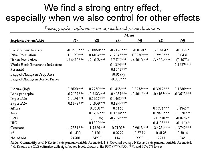
We find a strong entry effect, especially when we also control for other effects Demographic influences on agricultural price distortion Model (1) (2) (3) (4) (5) (6) Entry of new farmers Rural Population Urban Population World Bank Goverance Indicators Perennial Lagged Change in Crop Area Lagged Change in Border Prices -0. 0663*** 1. 1127*** -2. 4650*** -0. 0860*** 0. 4104*** -2. 1058*** -0. 2126*** -1. 7045*** 2. 7575*** 0. 1254*** -0. 1041*** (0. 0599) -0. 0037** -0. 0781* 1. 8950*** -4. 5010*** -0. 0804* 1. 2960*** -3. 6824*** -0. 1188* 0. 0431 (0. 5673) 0. 1627*** Income (log) Land per capita Importable Exportable Africa Asia LAC HIC Constant R 2 No. of obs. 0. 2620*** -0. 2525*** 0. 1154*** -0. 1673*** 0. 2230*** -0. 2423*** 0. 0665*** -0. 1959*** 0. 0600** 0. 3738*** (0. 0136) 0. 1822*** -1. 5356*** 0. 1501 24900 0. 1458*** -0. 6585*** 0. 1463*** -0. 1899*** 0. 1156 0. 3704*** -0. 2998***. -0. 7120** 0. 2779 1141 0. 3958*** -0. 4015*** 0. 3217*** -0. 4163*** 0. 1880*** -0. 3653*** -2. 9018*** 0. 3756 2233 0. 1701*** 0. 2880*** -0. 0670** 0. 4108*** -2. 4981*** 0. 4176 2233 0. 1861* 0. 3070*** -0. 0782* -0. 1154* -1. 3749*** 0. 5014 346 Explanatory variables -1. 7831*** 0. 1400 24900 Notes: Commodity level NRA is the dependent variable for models 1 -3. Covered average NRA is the dependent variable for models 4 -6. Results are OLS estimates with significance levels shown at the 99% (***), 95% (**), and 90% (*) levels.

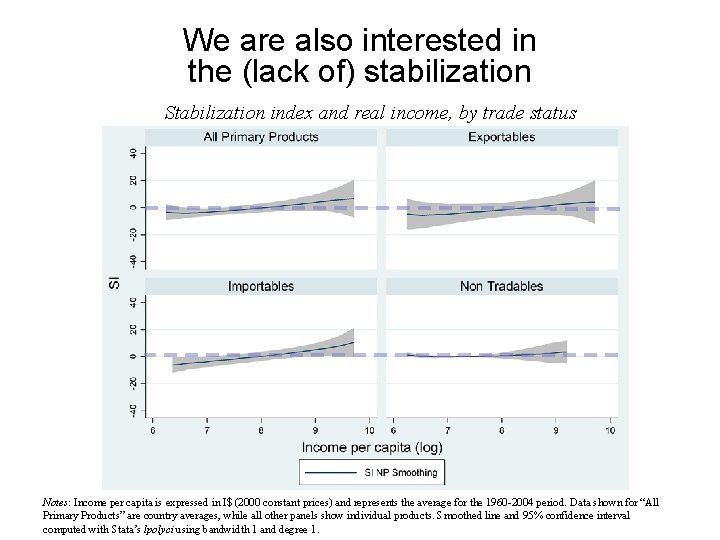
We are also interested in the (lack of) stabilization Stabilization index and real income, by trade status Notes: Income per capita is expressed in I$ (2000 constant prices) and represents the average for the 1960 -2004 period. Data shown for “All Primary Products” are country averages, while all other panels show individual products. Smoothed line and 95% confidence interval computed with Stata’s lpolyci using bandwidth 1 and degree 1.

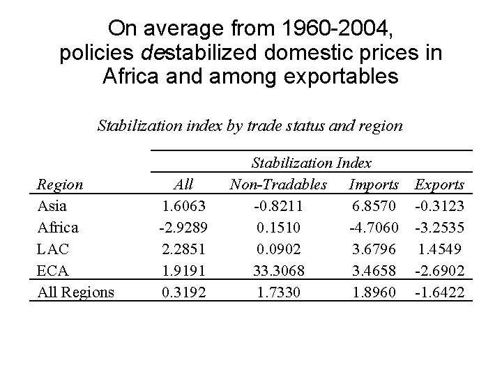
On average from 1960 -2004, policies destabilized domestic prices in Africa and among exportables Stabilization index by trade status and region Region Asia Africa LAC ECA All Regions All 1. 6063 -2. 9289 2. 2851 1. 9191 0. 3192 Stabilization Index Non-Tradables Imports -0. 8211 6. 8570 0. 1510 -4. 7060 0. 0902 3. 6796 33. 3068 3. 4658 1. 7330 1. 8960 Exports -0. 3123 -3. 2535 1. 4549 -2. 6902 -1. 6422

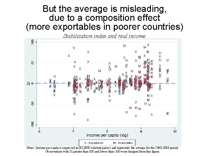
But the average is misleading, due to a composition effect (more exportables in poorer countries) Stabilization index and real income Notes: Income per capita is expressed in I$ (2000 constant prices) and represents the average for the 1960 -2004 period. Observations with SI greater than 100 and lower than -100 were dropped from this figure.

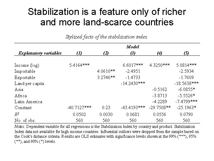
Stabilization is a feature only of richer and more land-scarce countries Stylized facts of the stabilization index Explanatory variables Income (log) Importable Exportable Land per capita Asia Africa Latin America Constant R 2 No. of obs. (1) (2) 5. 4164*** 4. 0610** 3. 2746** -40. 7127*** 0. 0502 560 0. 23 0. 0030 560 Model (3) (4) (5) 6. 6017*** 4. 3250*** 5. 0814*** -2. 4951 -2. 5934 -1. 4733 -1. 7609 -14. 2430*** -18. 5638*** -0. 5162 -6. 0855* -3. 8713 -5. 5526* -4. 2289 -7. 4799*** -43. 4193*** -29. 7508** -25. 1963* 0. 0681 0. 0556 0. 0790 560 560 Notes: Dependent variable for all regressions is the Stabilization Index by country and product. Stabilization Index data not available for high income countries. Influential outliers were dropped from the sample based on the Cook's distance criteria. Results are OLS estimates with significance levels shown at the 99% (***), 95% (**), and 90% (*) levels.

Some conclusions • The three stylized facts w. r. t. income level, trade direction and land abundance are robust but explain only a small fraction of variance • The six specific political economy mechanisms generally add explanatory power to the stylized facts, rather than explaining them. (Only governance could account for a large fraction of the income effect. ) • Main novelty here is effect of new farmers’ entry; effect is same or larger when instrumented, and it adds explanatory power as well as helping to accounts for income effect • Main surprise here is (lack of) stabilization, except in the richer and more land-scarce countries