Exploring Data Measures of Center and Spread Adapted

Exploring Data Measures of Center and Spread Adapted from Ms. Namad

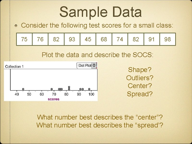
Sample Data Consider the following test scores for a small class: 75 76 82 93 45 68 74 82 91 Plot the data and describe the SOCS: Shape? Outliers? Center? Spread? What number best describes the “center”? What number best describes the “spread’? 98

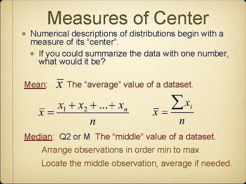
Measures of Center Numerical descriptions of distributions begin with a measure of its “center”. If you could summarize the data with one number, what would it be? Mean: The “average” value of a dataset. Median: Q 2 or M The “middle” value of a dataset. Arrange observations in order min to max Locate the middle observation, average if needed.

Mean vs. Median The mean and the median are the most common measures of center. If a distribution is perfectly symmetric, the mean and the median are the same. The mean is not resistant to outliers. You must decide which number is the most appropriate description of the center. . .

Measures of Spread Variability is the key to Statistics. Without variability, there would be no need for the subject. When describing data, never rely on center alone. Measures of Spread: Range - {rarely used. . . why? } Quartiles - Inter. Quartile Range {IQR=Q 3 -Q 1} Variance and Standard Deviation {var and sx} Like Measures of Center, you must choose the most appropriate measure of spread.

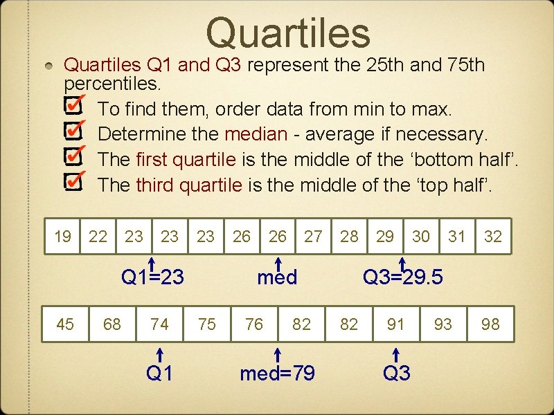
Quartiles Q 1 and Q 3 represent the 25 th and 75 th percentiles. To find them, order data from min to max. Determine the median - average if necessary. The first quartile is the middle of the ‘bottom half’. The third quartile is the middle of the ‘top half’. 19 22 23 23 23 Q 1=23 45 68 74 Q 1 26 26 27 28 med 75 76 82 med=79 29 30 31 32 Q 3=29. 5 82 91 Q 3 93 98

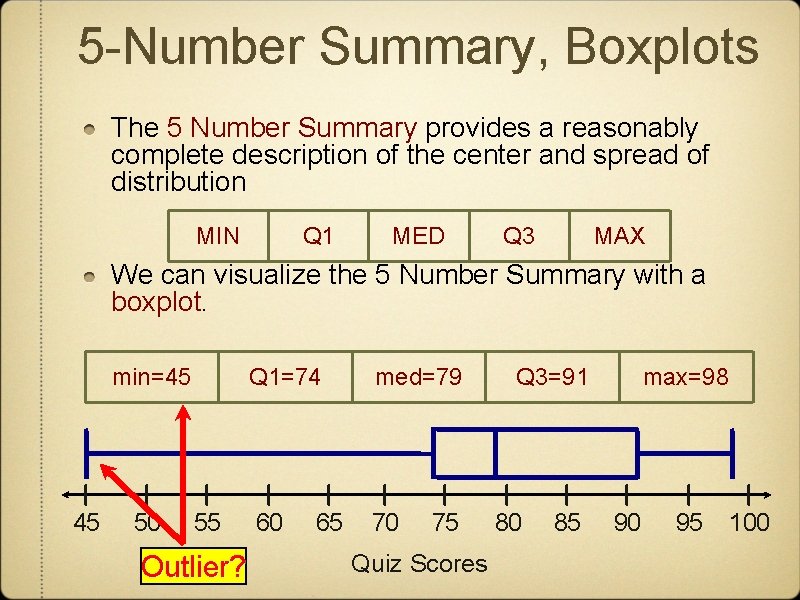
5 -Number Summary, Boxplots The 5 Number Summary provides a reasonably complete description of the center and spread of distribution MIN Q 1 MED Q 3 MAX We can visualize the 5 Number Summary with a boxplot. min=45 45 50 55 Outlier? Q 1=74 med=79 60 70 65 75 Quiz Scores Q 3=91 80 85 max=98 90 95 100

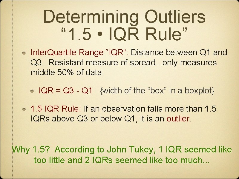
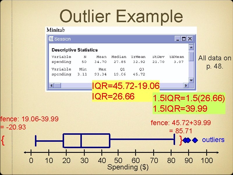
Determining Outliers “ 1. 5 • IQR Rule” Inter. Quartile Range “IQR”: Distance between Q 1 and Q 3. Resistant measure of spread. . . only measures middle 50% of data. IQR = Q 3 - Q 1 {width of the “box” in a boxplot} 1. 5 IQR Rule: If an observation falls more than 1. 5 IQRs above Q 3 or below Q 1, it is an outlier. Why 1. 5? According to John Tukey, 1 IQR seemed like too little and 2 IQRs seemed like too much. . .

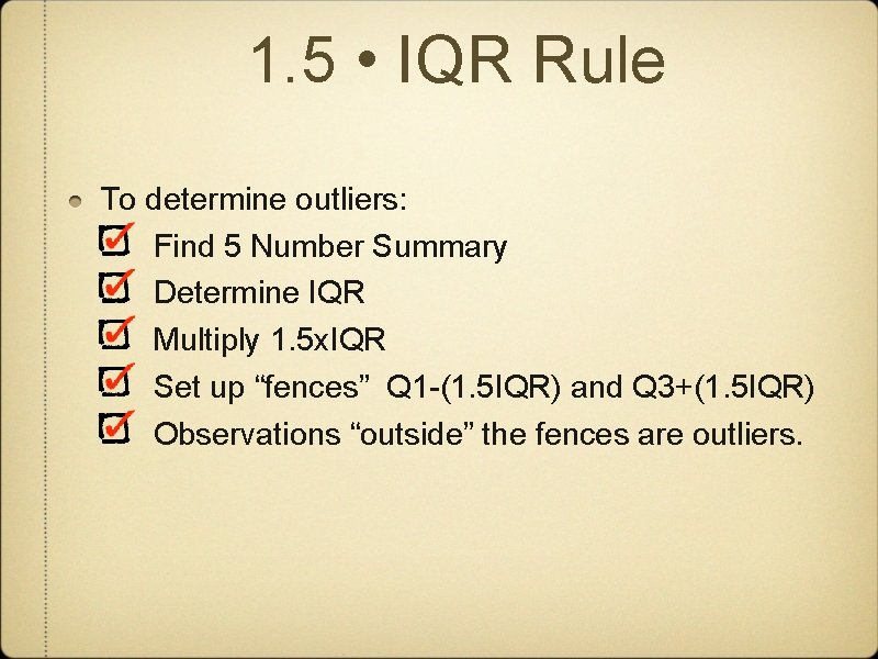
1. 5 • IQR Rule To determine outliers: Find 5 Number Summary Determine IQR Multiply 1. 5 x. IQR Set up “fences” Q 1 -(1. 5 IQR) and Q 3+(1. 5 IQR) Observations “outside” the fences are outliers.

Outlier Example All data on p. 48. IQR=45. 72 -19. 06 IQR=26. 66 1. 5 IQR=1. 5(26. 66) 1. 5 IQR=39. 99 fence: 19. 06 -39. 99 = -20. 93 fence: 45. 72+39. 99 = 85. 71 outliers } { 0 10 20 30 40 50 60 70 Spending ($) 80 90 100

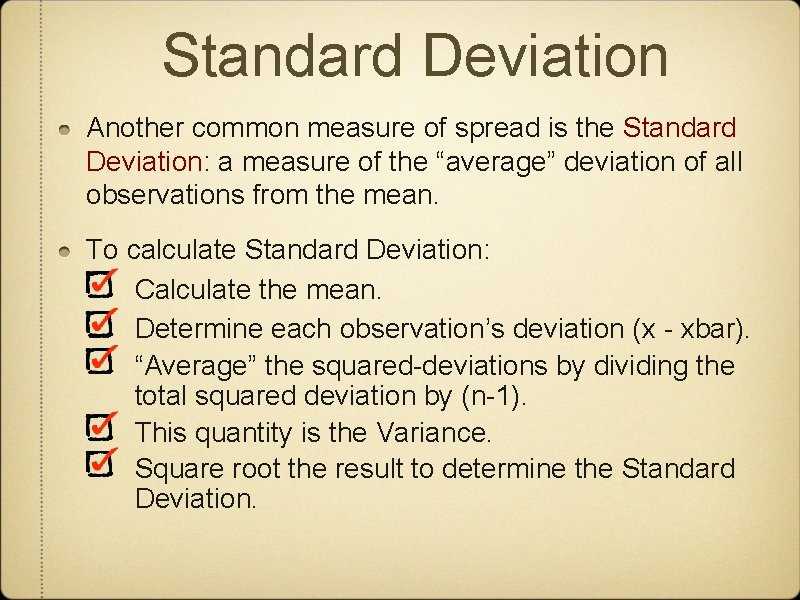
Standard Deviation Another common measure of spread is the Standard Deviation: a measure of the “average” deviation of all observations from the mean. To calculate Standard Deviation: Calculate the mean. Determine each observation’s deviation (x - xbar). “Average” the squared-deviations by dividing the total squared deviation by (n-1). This quantity is the Variance. Square root the result to determine the Standard Deviation.

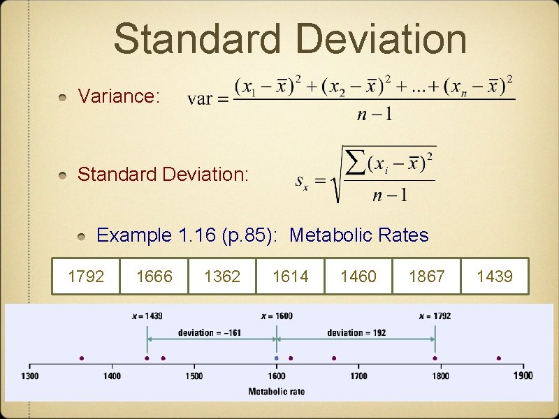
Standard Deviation Variance: Standard Deviation: Example 1. 16 (p. 85): Metabolic Rates 1792 1666 1362 1614 1460 1867 1439

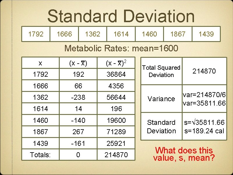
Standard Deviation 1792 1666 1362 1614 1460 1867 1439 Metabolic Rates: mean=1600 x (x - x)2 1792 192 36864 1666 66 4356 1362 -238 56644 1614 14 196 1460 -140 19600 1867 267 71289 1439 -161 25921 Totals: 0 214870 Total Squared Deviation 214870 Variance var=214870/6 var=35811. 66 Standard Deviation s=√ 35811. 66 s=189. 24 cal What does this value, s, mean?

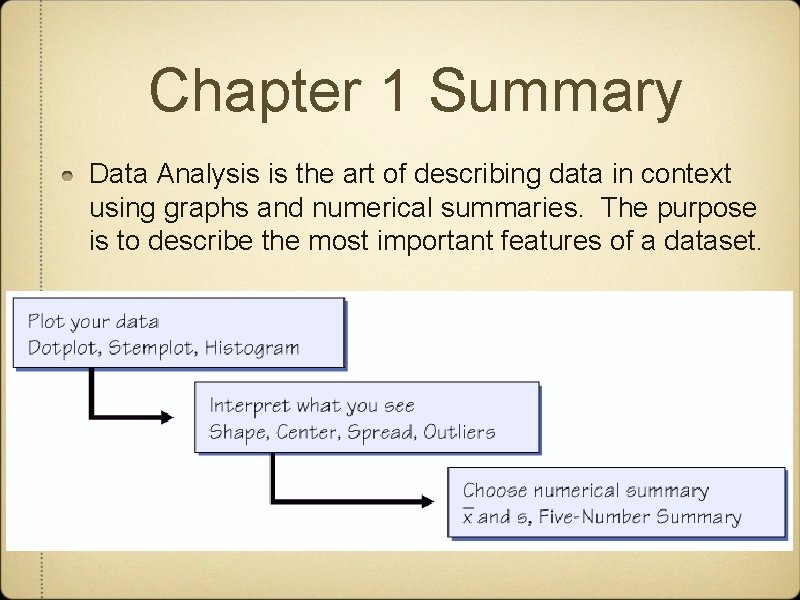
Chapter 1 Summary Data Analysis is the art of describing data in context using graphs and numerical summaries. The purpose is to describe the most important features of a dataset.