Experimentos Fatoriais do tipo k 2 Captulo 6

Experimentos Fatoriais do tipo k 2 Capítulo 6

6. 5 Unreplicated 2 k Factorial Designs • These are 2 k factorial designs with one observation at each corner of the “cube” • An unreplicated 2 k factorial design is also sometimes called a “single replicate” of the 2 k • These designs are very widely used • Risks…if there is only one observation at each corner, is there a chance of unusual response observations spoiling the results? • Modeling “noise”?

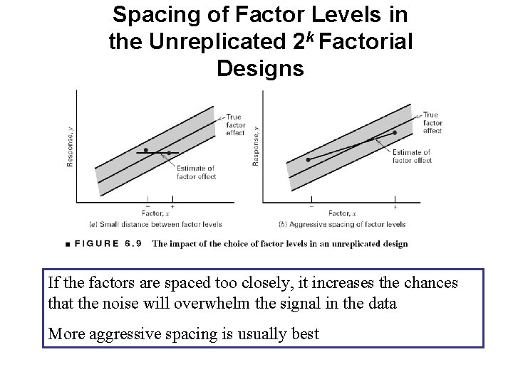
Spacing of Factor Levels in the Unreplicated 2 k Factorial Designs If the factors are spaced too closely, it increases the chances that the noise will overwhelm the signal in the data More aggressive spacing is usually best

Unreplicated 2 k Factorial Designs • Lack of replication causes potential problems in statistical testing – Replication admits an estimate of “pure error” (a better phrase is an internal estimate of error) – With no replication, fitting the full model results in zero degrees of freedom for error • Potential solutions to this problem – Pooling high-order interactions to estimate error – Normal probability plotting of effects (Daniels, 1959) – Other methods…see text

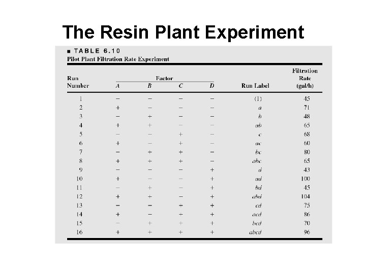
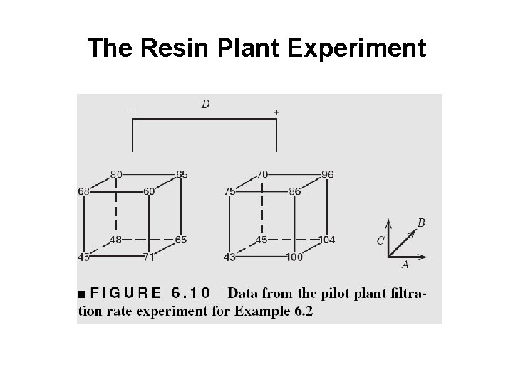
Example of an Unreplicated 2 k Design • A 24 factorial was used to investigate the effects of four factors on the filtration rate of a resin • The factors are A = temperature, B = pressure, C = mole ratio, D= stirring rate • Experiment was performed in a pilot plant

The Resin Plant Experiment

The Resin Plant Experiment

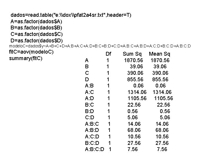
dados=read. table("e: \dox\pfat 2 a 4 sr. txt", header=T) A=as. factor(dados$A) B=as. factor(dados$B) C=as. factor(dados$C) D=as. factor(dados$D) modelo. C=dados$y~A+B+C+D+A: B+A: C+A: D+B: C+B: D+C: D+A: B: C+A: B: D+A: C: D+B: C: D+A: B: C: D fit. C=aov(modelo. C) summary(fit. C) Df A 1 B 1 C 1 D 1 A: B 1 A: C 1 A: D 1 B: C 1 B: D 1 C: D 1 A: B: C 1 A: B: D 1 A: C: D 1 B: C: D 1 A: B: C: D 1 Sum Sq Mean Sq 1870. 56 39. 06 390. 06 855. 56 0. 06 1314. 06 1105. 56 22. 56 0. 56 5. 06 14. 06 68. 06 10. 56 27. 56

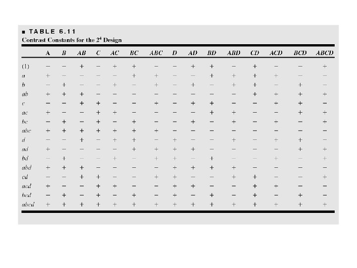
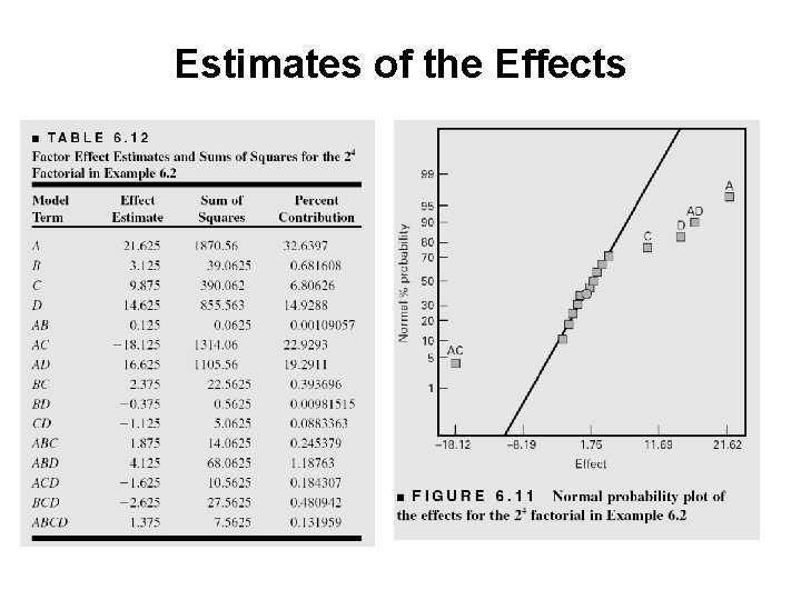
Estimates of the Effects

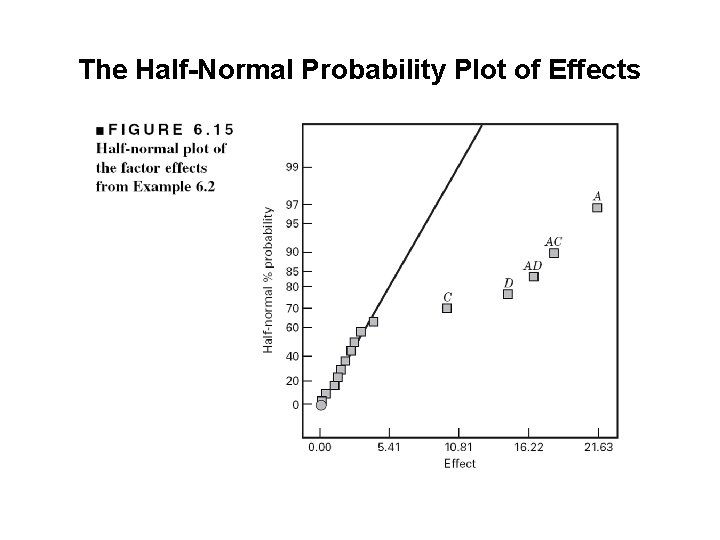
The Half-Normal Probability Plot of Effects

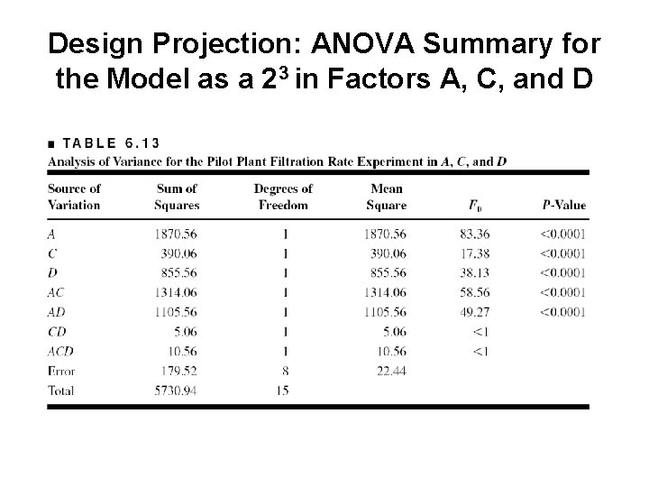
Design Projection: ANOVA Summary for the Model as a 23 in Factors A, C, and D

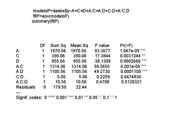
modelo. P=dados$y~A+C+D+A: C+A: D+C: D+A: C: D fit. P=aov(modelo. P) summary(fit. P) Df Sum Sq Mean Sq 1 1870. 56 1 390. 06 1 855. 56 1 1314. 06 1 1105. 56 1 5. 06 1 10. 56 8 179. 50 22. 44 F value 83. 3677 17. 3844 38. 1309 58. 5655 49. 2730 0. 2256 0. 4708 A C D A: C A: D C: D A: C: D Residuals --Signif. codes: 0 ‘***’ 0. 001 ‘**’ 0. 01 ‘*’ 0. 05 ‘. ’ 0. 1 ‘ ’ 1 Pr(>F) 1. 667 e-05 *** 0. 0031244 ** 0. 0002666 *** 6. 001 e-05 *** 0. 0001105 *** 0. 6474830 0. 5120321

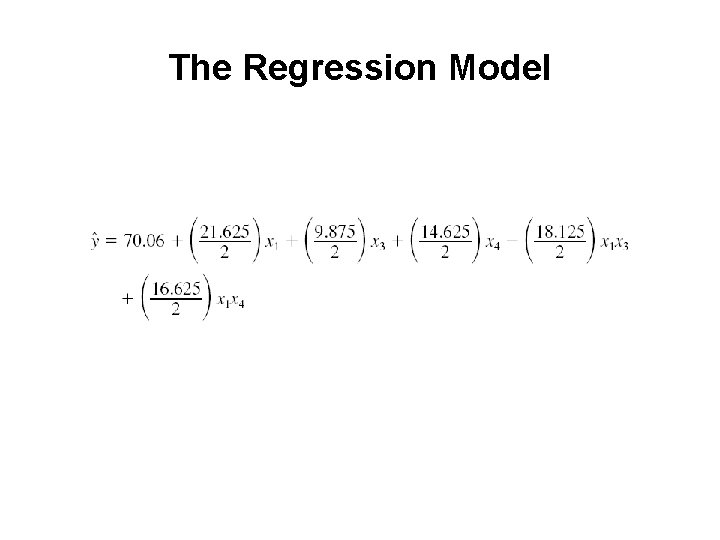
The Regression Model

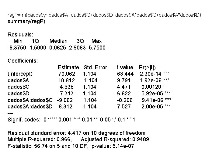
reg. P=lm(dados$y~dados$A+dados$C+dados$D+dados$A*dados$C+dados$A*dados$D) summary(reg. P) Residuals: Min 1 Q Median 3 Q Max -6. 3750 -1. 5000 0. 0625 2. 9063 5. 7500 Coefficients: Estimate Std. Error t value Pr(>|t|) (Intercept) 70. 062 1. 104 63. 444 2. 30 e-14 *** dados$A 10. 812 1. 104 9. 791 1. 93 e-06 *** dados$C 4. 938 1. 104 4. 471 0. 00120 ** dados$D 7. 313 1. 104 6. 622 5. 92 e-05 *** dados$A: dados$C -9. 062 1. 104 -8. 206 9. 41 e-06 *** dados$A: dados$D 8. 312 1. 104 7. 527 2. 00 e-05 *** --Signif. codes: 0 ‘***’ 0. 001 ‘**’ 0. 01 ‘*’ 0. 05 ‘. ’ 0. 1 ‘ ’ 1 Residual standard error: 4. 417 on 10 degrees of freedom Multiple R-squared: 0. 966, Adjusted R-squared: 0. 9489 F-statistic: 56. 74 on 5 and 10 DF, p-value: 5. 14 e-07

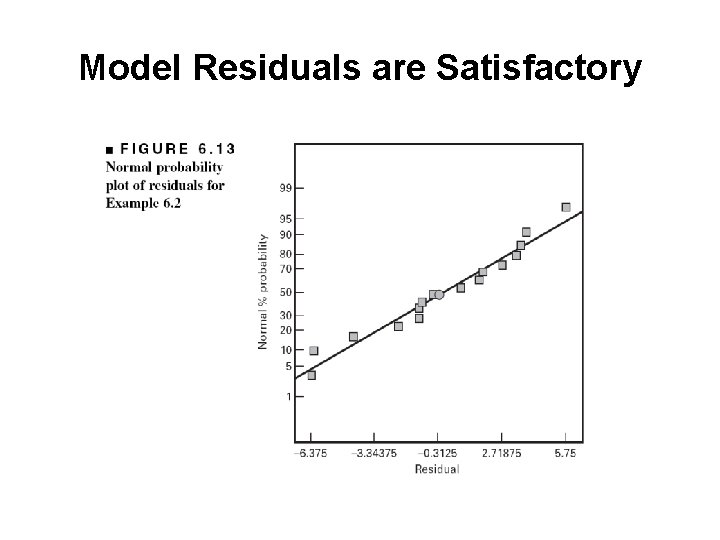
Model Residuals are Satisfactory

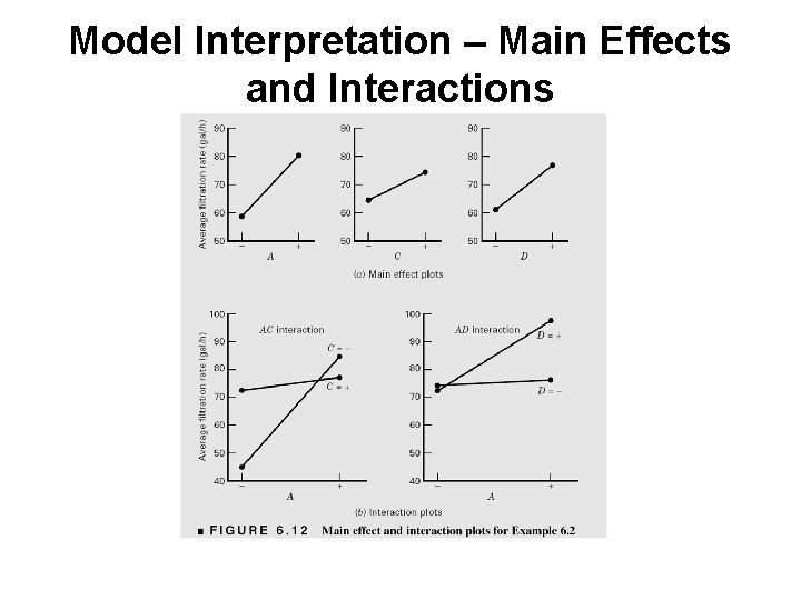
Model Interpretation – Main Effects and Interactions

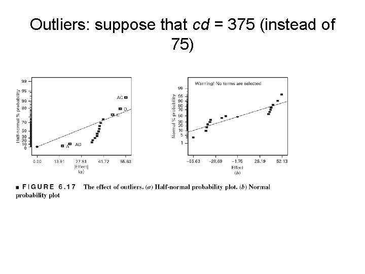
Outliers: suppose that cd = 375 (instead of 75)

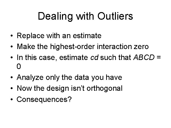
Dealing with Outliers • Replace with an estimate • Make the highest-order interaction zero • In this case, estimate cd such that ABCD = 0 • Analyze only the data you have • Now the design isn’t orthogonal • Consequences?

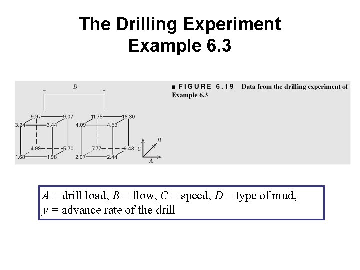
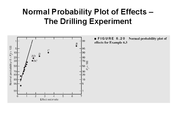
The Drilling Experiment Example 6. 3 A = drill load, B = flow, C = speed, D = type of mud, y = advance rate of the drill

Normal Probability Plot of Effects – The Drilling Experiment

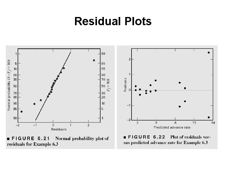
Residual Plots

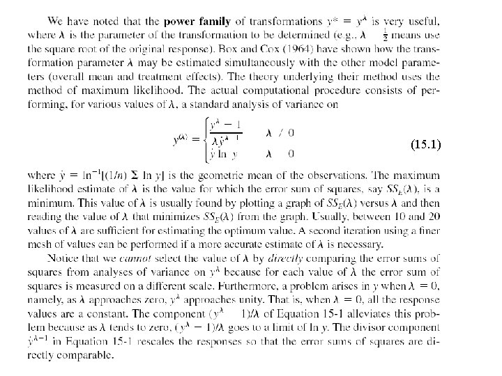
Residual Plots • The residual plots indicate that there are problems with the equality of variance assumption • The usual approach to this problem is to employ a transformation on the response • Power family transformations are widely used Transformations are typically performed to – Stabilize variance – Induce at least approximate normality – Simplify the model

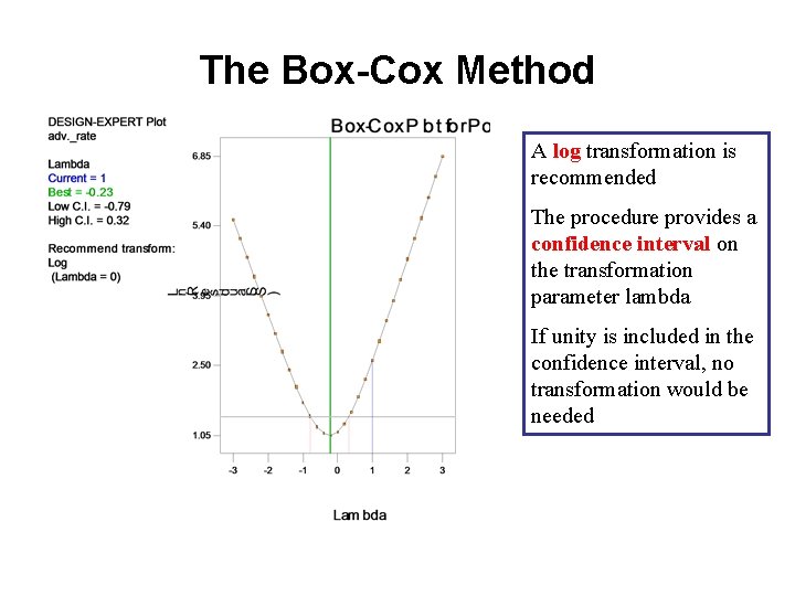
Selecting a Transformation • Empirical selection of lambda • Prior (theoretical) knowledge or experience can often suggest the form of a transformation • Analytical selection of lambda…the Box-Cox (1964) method (simultaneously estimates the model parameters and the transformation parameter lambda) • Box-Cox method implemented in Design. Expert

(15. 1)

The Box-Cox Method A log transformation is recommended The procedure provides a confidence interval on the transformation parameter lambda If unity is included in the confidence interval, no transformation would be needed

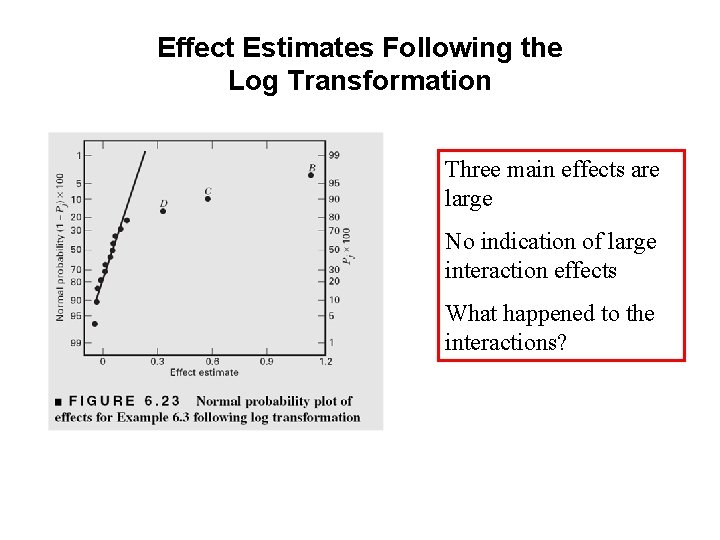
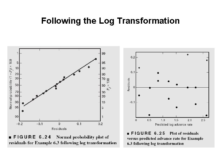
Effect Estimates Following the Log Transformation Three main effects are large No indication of large interaction effects What happened to the interactions?

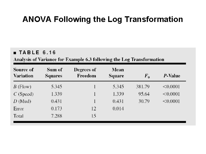
ANOVA Following the Log Transformation

Following the Log Transformation

The Log Advance Rate Model • Is the log model “better”? • We would generally prefer a simpler model in a transformed scale to a more complicated model in the original metric • What happened to the interactions? • Sometimes transformations provide insight into the underlying mechanism

Other Examples of Unreplicated 2 k Designs • The sidewall panel experiment (Example 6. 4, pg. 245) – Two factors affect the mean number of defects – A third factor affects variability – Residual plots were useful in identifying the dispersion effect • The oxidation furnace experiment (Example 6. 5, pg. 245) – Replicates versus repeat (or duplicate) observations? – Modeling within-run variability

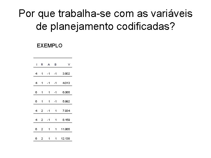
Por que trabalha-se com as variáveis de planejamento codificadas? EXEMPLO I R A B V 4 1 -1 -1 3. 802 4 1 -1 -1 4. 013 6 1 1 -1 6. 065 6 1 1 -1 5. 992 4 2 -1 1 7. 934 4 2 -1 1 8. 159 6 2 1 1 11. 865 6 2 1 1 12. 138

• Na análise com as variáveis codificadas, as magnitudes dos coeficientes do modelo são diretamente comparáveis, isto é, elas são adimensionais, e medem os efeitos da variação de cada fator de planejamento sobre um intervalo unitário. • Além disso, são todas estimadas com a mesma precisão. • Variáveis codificadas são muito efetivas para determinar o tamanho relativo dos efeitos dos fatores.

• Em geral, os coeficientes obtidos usandose as unidades originais não são diretamente comparáveis, mas eles podem ter significado físico. • Em quase todas as situações, a análise codificada é preferível.