ENGR 43235323 Digital and Analog Communication Ch 8

ENGR 4323/5323 Digital and Analog Communication Ch 8 Fundamentals of Probability Theory Engineering and Physics University of Central Oklahoma Dr. Mohamed Bingabr

Chapter Outline • Concept of Probability • Random Variables • Statistical Averages (MEANS) • Correlation • Linear Mean Square Estimation • Sum of Random Variables • Central Limit Theorem 2

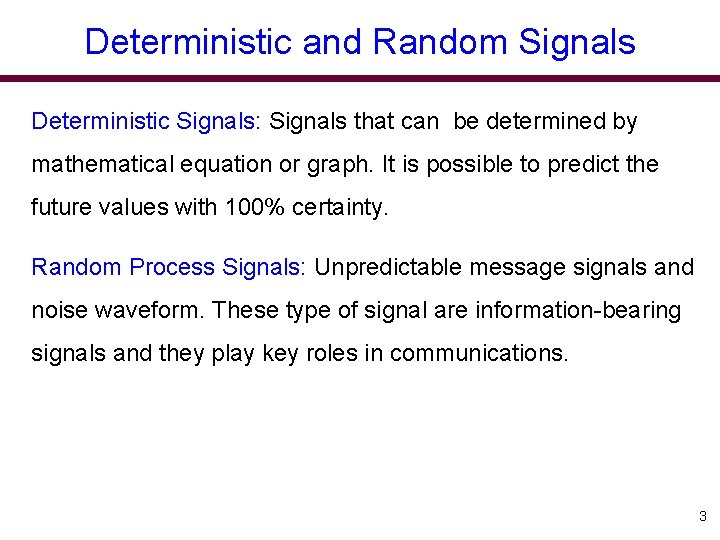
Deterministic and Random Signals Deterministic Signals: Signals that can be determined by mathematical equation or graph. It is possible to predict the future values with 100% certainty. Random Process Signals: Unpredictable message signals and noise waveform. These type of signal are information-bearing signals and they play key roles in communications. 3

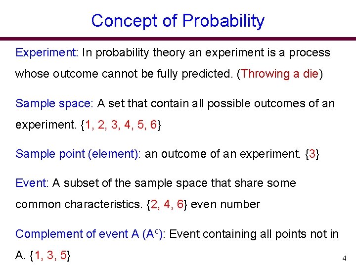
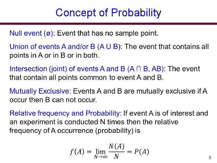
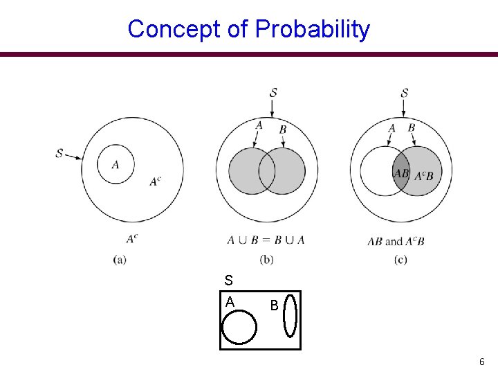
Concept of Probability Experiment: In probability theory an experiment is a process whose outcome cannot be fully predicted. (Throwing a die) Sample space: A set that contain all possible outcomes of an experiment. {1, 2, 3, 4, 5, 6} Sample point (element): an outcome of an experiment. {3} Event: A subset of the sample space that share some common characteristics. {2, 4, 6} even number Complement of event A (Ac): Event containing all points not in A. {1, 3, 5} 4

Concept of Probability 5

Concept of Probability S A B 6

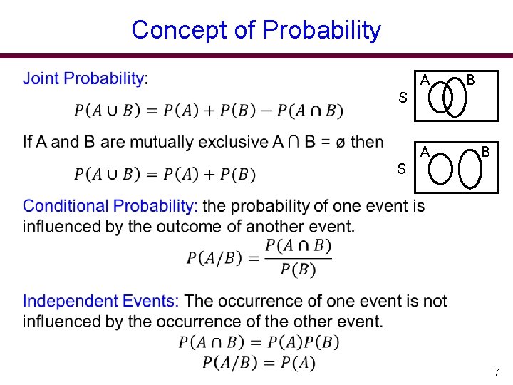
Concept of Probability A B S 7

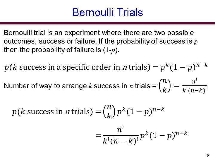
Bernoulli Trials 8

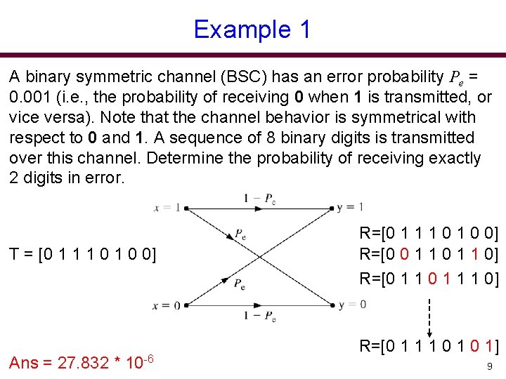
Example 1 A binary symmetric channel (BSC) has an error probability Pe = 0. 001 (i. e. , the probability of receiving 0 when 1 is transmitted, or vice versa). Note that the channel behavior is symmetrical with respect to 0 and 1. A sequence of 8 binary digits is transmitted over this channel. Determine the probability of receiving exactly 2 digits in error. T = [0 1 1 1 0 0] Ans = 27. 832 * 10 -6 R=[0 1 1 1 0 0] R=[0 0 1 1 0] R=[0 1 1 1 0 1] 9

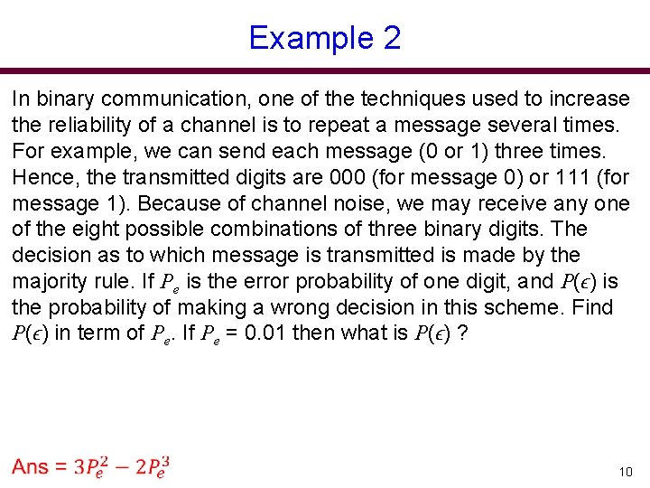
Example 2 In binary communication, one of the techniques used to increase the reliability of a channel is to repeat a message several times. For example, we can send each message (0 or 1) three times. Hence, the transmitted digits are 000 (for message 0) or 111 (for message 1). Because of channel noise, we may receive any one of the eight possible combinations of three binary digits. The decision as to which message is transmitted is made by the majority rule. If Pe is the error probability of one digit, and P(ϵ) is the probability of making a wrong decision in this scheme. Find P(ϵ) in term of Pe. If Pe = 0. 01 then what is P(ϵ) ? 10

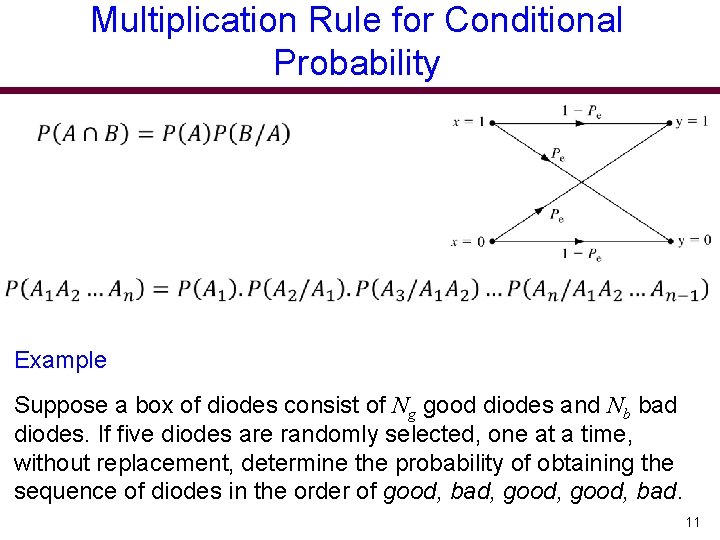
Multiplication Rule for Conditional Probability Example Suppose a box of diodes consist of Ng good diodes and Nb bad diodes. If five diodes are randomly selected, one at a time, without replacement, determine the probability of obtaining the sequence of diodes in the order of good, bad, good, bad. 11

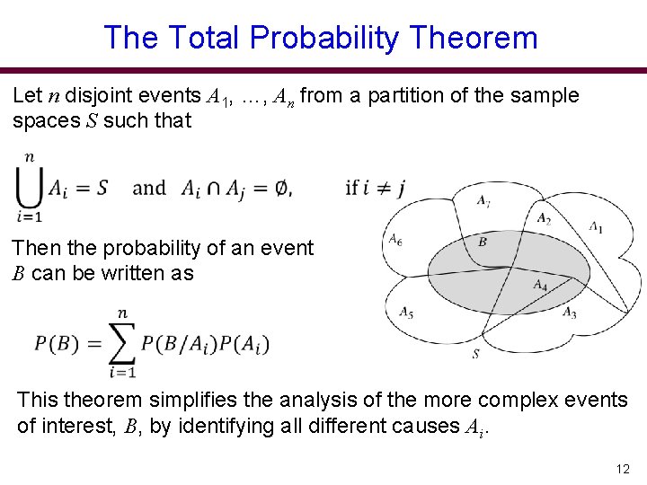
The Total Probability Theorem Let n disjoint events A 1, …, An from a partition of the sample spaces S such that Then the probability of an event B can be written as This theorem simplifies the analysis of the more complex events of interest, B, by identifying all different causes Ai. 12

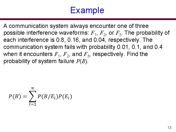
Example A communication system always encounter one of three possible interference waveforms: F 1, F 2, or F 3. The probability of each interference is 0. 8, 0. 16, and 0. 04, respectively. The communication system fails with probability 0. 01, 0. 1, and 0. 4 when it encounters F 1, F 2, and F 3, respectively. Find the probability of system failure P(B). 13

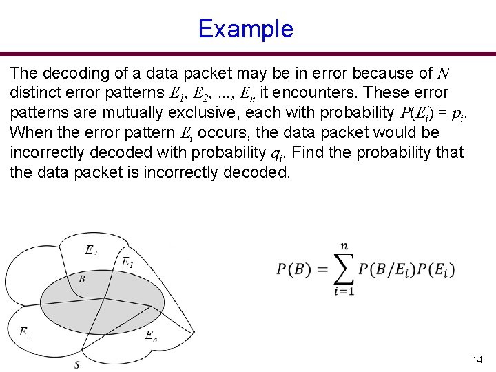
Example The decoding of a data packet may be in error because of N distinct error patterns E 1, E 2, …, En it encounters. These error patterns are mutually exclusive, each with probability P(Ei) = pi. When the error pattern Ei occurs, the data packet would be incorrectly decoded with probability qi. Find the probability that the data packet is incorrectly decoded. 14

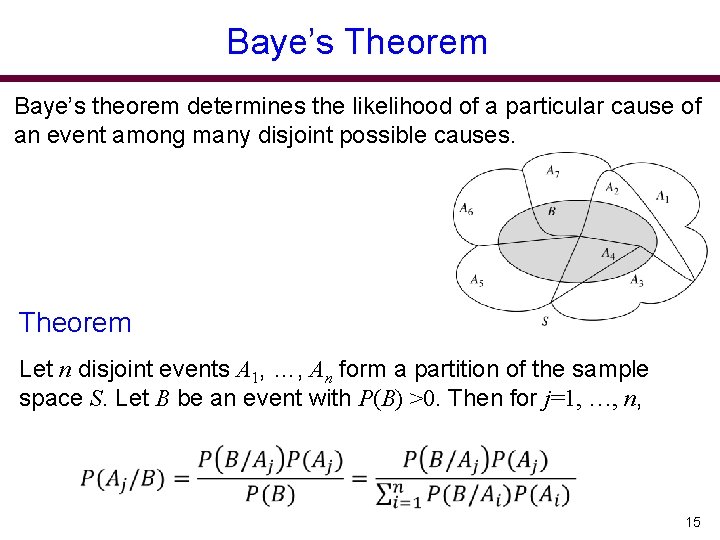
Baye’s Theorem Baye’s theorem determines the likelihood of a particular cause of an event among many disjoint possible causes. Theorem Let n disjoint events A 1, …, An form a partition of the sample space S. Let B be an event with P(B) >0. Then for j=1, …, n, 15

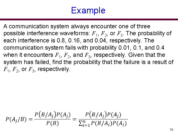
Example A communication system always encounter one of three possible interference waveforms: F 1, F 2, or F 3. The probability of each interference is 0. 8, 0. 16, and 0. 04, respectively. The communication system fails with probability 0. 01, 0. 1, and 0. 4 when it encounters F 1, F 2, and F 3, respectively. Given that the system has failed, find the probability that the failure is a result of F 1, F 2, or F 3, respectively. 16

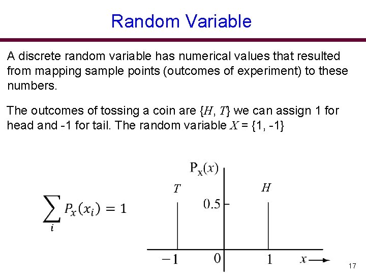
Random Variable A discrete random variable has numerical values that resulted from mapping sample points (outcomes of experiment) to these numbers. The outcomes of tossing a coin are {H, T} we can assign 1 for head and -1 for tail. The random variable X = {1, -1} T H 17

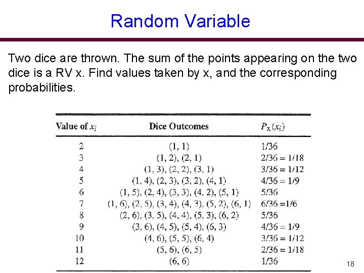
Random Variable Two dice are thrown. The sum of the points appearing on the two dice is a RV x. Find values taken by x, and the corresponding probabilities. 18

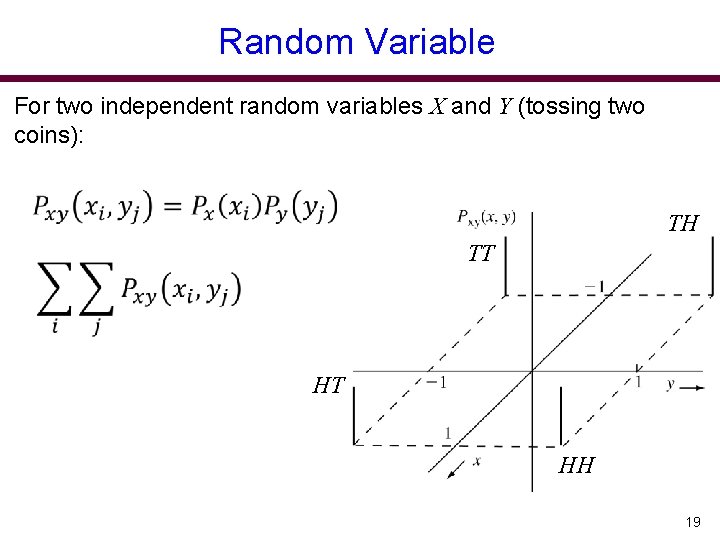
Random Variable For two independent random variables X and Y (tossing two coins): TH TT HT HH 19

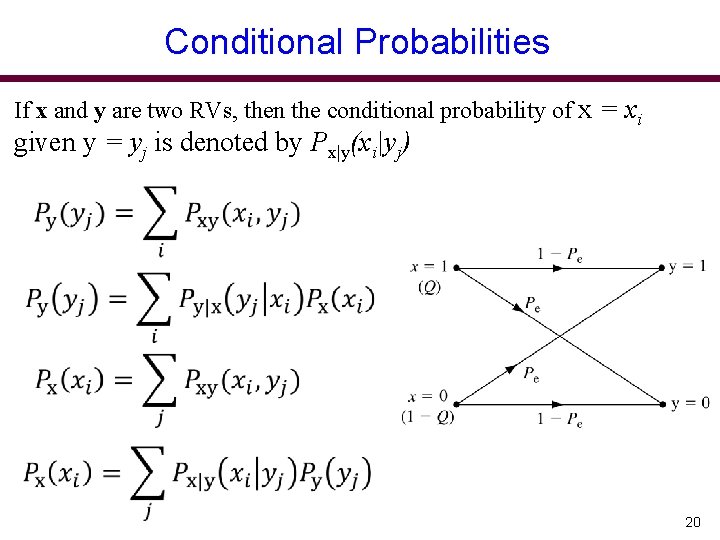
Conditional Probabilities If x and y are two RVs, then the conditional probability of x = xi given y = yj is denoted by Px|y(xi|yj) 20

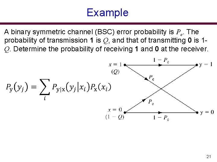
Example A binary symmetric channel (BSC) error probability is Pe. The probability of transmission 1 is Q, and that of transmitting 0 is 1 Q. Determine the probability of receiving 1 and 0 at the receiver. 21

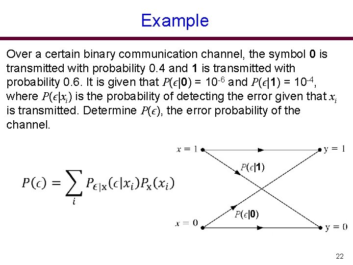
Example Over a certain binary communication channel, the symbol 0 is transmitted with probability 0. 4 and 1 is transmitted with probability 0. 6. It is given that P(ϵ|0) = 10 -6 and P(ϵ|1) = 10 -4, where P(ϵ|xi) is the probability of detecting the error given that xi is transmitted. Determine P(ϵ), the error probability of the channel. P(ϵ|1) P(ϵ|0) 22

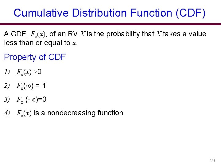
Cumulative Distribution Function (CDF) A CDF, Fx(x), of an RV X is the probability that X takes a value less than or equal to x. Property of CDF 1) Fx(x) 0 2) Fx( ) = 1 3) Fx (- )=0 4) Fx(x) is a nondecreasing function. 23

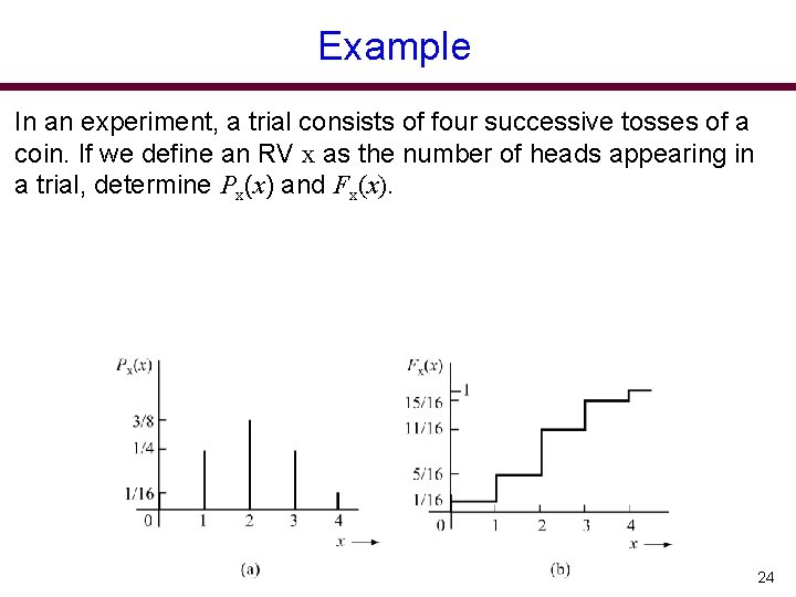
Example In an experiment, a trial consists of four successive tosses of a coin. If we define an RV x as the number of heads appearing in a trial, determine Px(x) and Fx(x). 24

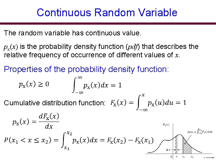
Continuous Random Variable The random variable has continuous value. px(x) is the probability density function (pdf) that describes the relative frequency of occurrence of different values of x. Properties of the probability density function: Cumulative distribution function: 25

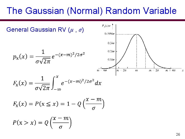
The Gaussian (Normal) Random Variable General Gaussian RV (µ , σ) 26

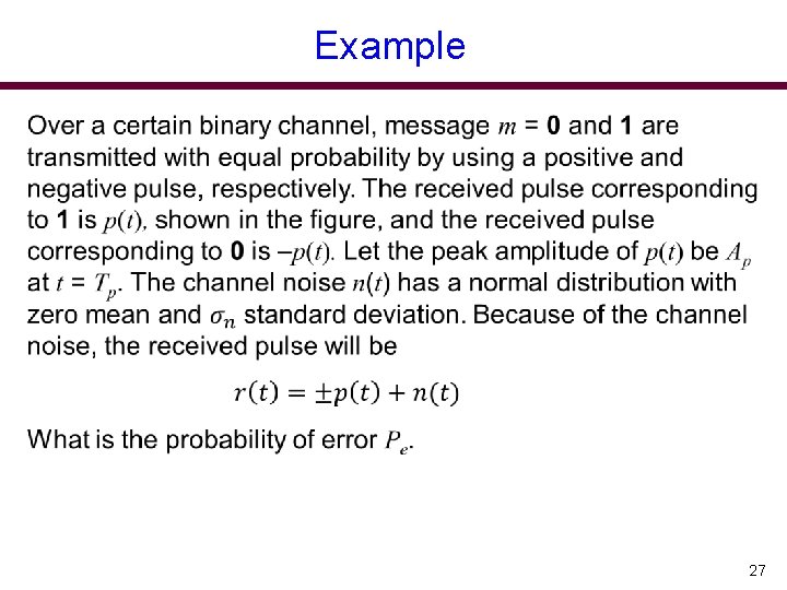
Example 27

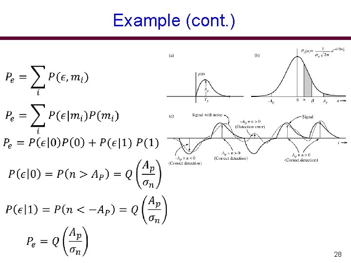
Example (cont. ) 28

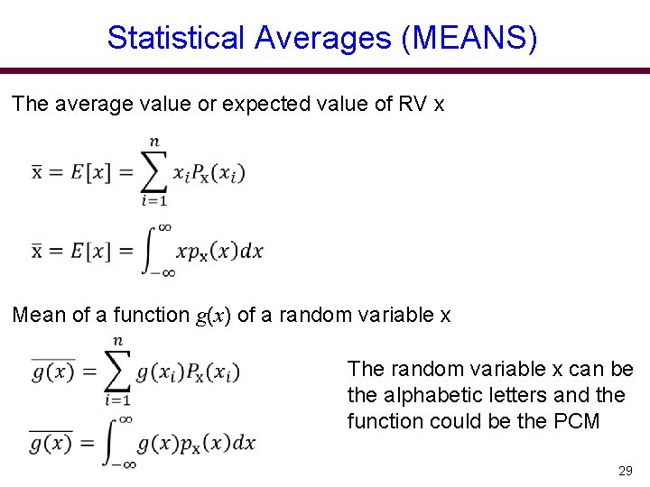
Statistical Averages (MEANS) The average value or expected value of RV x Mean of a function g(x) of a random variable x The random variable x can be the alphabetic letters and the function could be the PCM 29

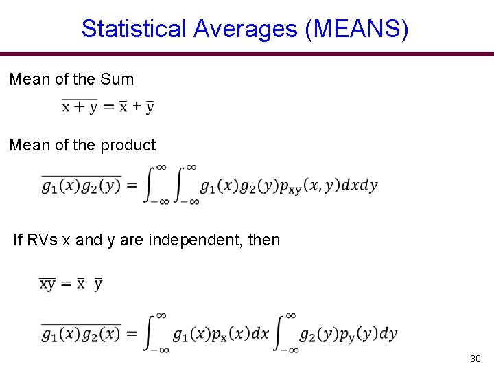
Statistical Averages (MEANS) Mean of the Sum Mean of the product If RVs x and y are independent, then 30

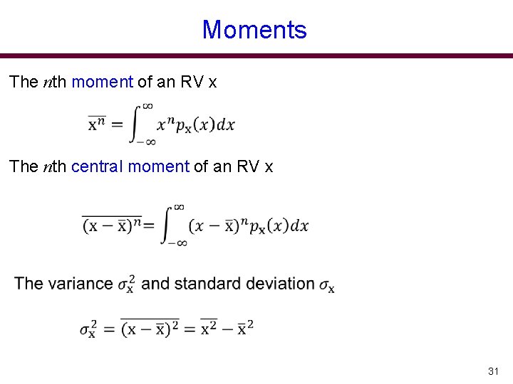
Moments The nth moment of an RV x The nth central moment of an RV x 31

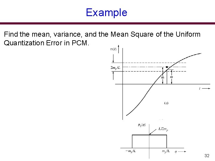
Example Find the mean, variance, and the Mean Square of the Uniform Quantization Error in PCM. 32