Electron Identification with Neural Networks Dominique Godin Kazuya

Electron Identification with Neural Networks Dominique Godin Kazuya Mochizuki Sergey Panitkin Emre Onur Kahya Alain Tapp Etienne Dreyer Jean-François Arguin Otilia Ducu Julien Maurer Ioan-Mihail Dinu Chloe Lefebvre Olivier Denis 2020 -09 -09

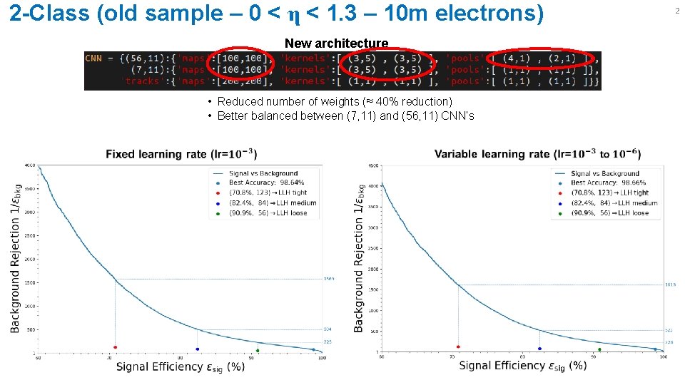
2 -Class (old sample – 0 < η < 1. 3 – 10 m electrons) New architecture • Reduced number of weights (≈ 40% reduction) • Better balanced between (7, 11) and (56, 11) CNN’s 2

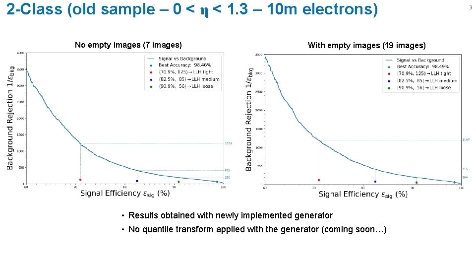
2 -Class (old sample – 0 < η < 1. 3 – 10 m electrons) No empty images (7 images) With empty images (19 images) • Results obtained with newly implemented generator • No quantile transform applied with the generator (coming soon…) 3

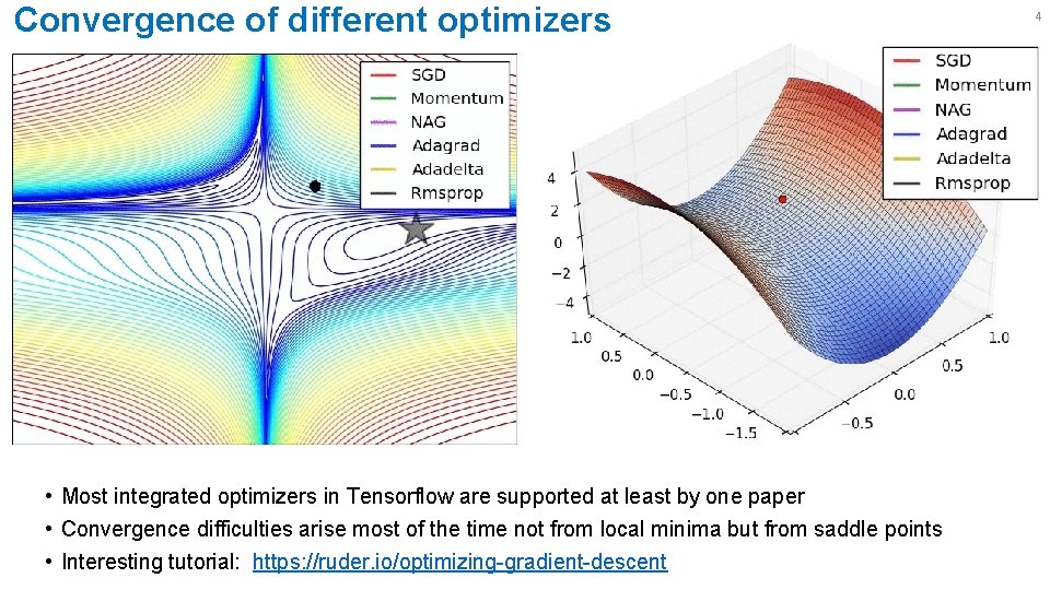
Convergence of different optimizers • Most integrated optimizers in Tensorflow are supported at least by one paper • Convergence difficulties arise most of the time not from local minima but from saddle points • Interesting tutorial: https: //ruder. io/optimizing-gradient-descent 4

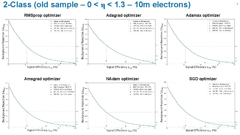
2 -Class (old sample – 0 < η < 1. 3 – 10 m electrons) RMSprop optimizer Adagrad optimizer Adamax optimizer Amsgrad optimizer NAdam optimizer SGD optimizer 5

6 Backup Material

Project Group Members • This project is largely supported by IVADO • Many thanks to the Copenhagen group for providing us with data samples 7

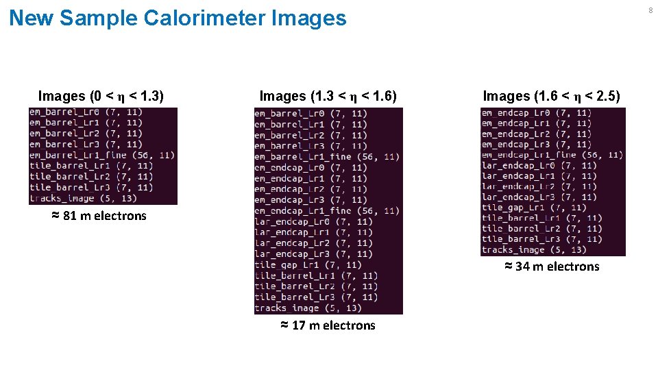
8 New Sample Calorimeter Images (0 < η < 1. 3) Images (1. 3 < η < 1. 6) Images (1. 6 < η < 2. 5) ≈ 81 m electrons ≈ 34 m electrons ≈ 17 m electrons

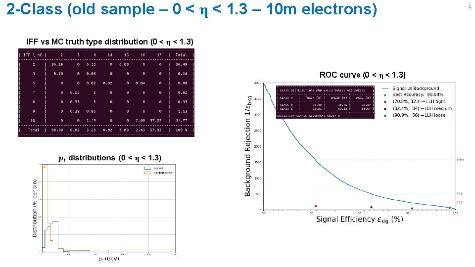
2 -Class (old sample – 0 < η < 1. 3 – 10 m electrons) IFF vs MC truth type distribution (0 < η < 1. 3) ROC curve (0 < η < 1. 3) 9

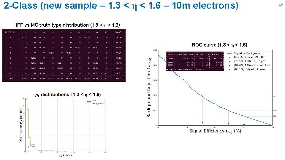
2 -Class (new sample – 1. 3 < η < 1. 6 – 10 m electrons) IFF vs MC truth type distribution (1. 3 < η < 1. 6) ROC curve (1. 3 < η < 1. 6) 10

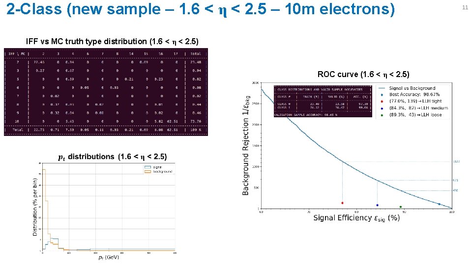
2 -Class (new sample – 1. 6 < η < 2. 5 – 10 m electrons) IFF vs MC truth type distribution (1. 6 < η < 2. 5) ROC curve (1. 6 < η < 2. 5) 11

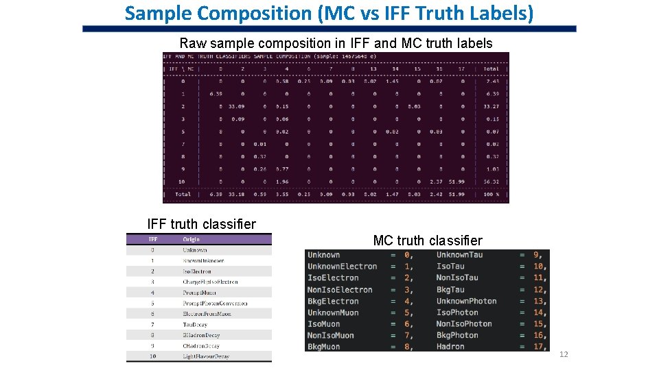
Sample Composition (MC vs IFF Truth Labels) Raw sample composition in IFF and MC truth labels IFF truth classifier MC truth classifier 12

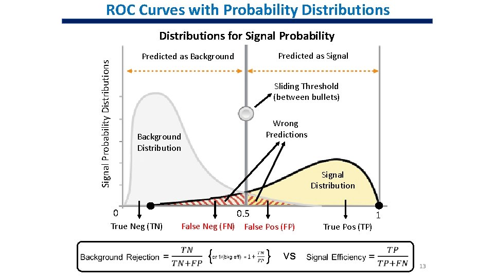
ROC Curves with Probability Distributions for Signal Probability Predicted as Signal Probability Distributions Predicted as Background Sliding Threshold (between bullets) Wrong Predictions Background Distribution Signal Distribution 0 True Neg (TN) 0. 5 False Neg (FN) False Pos (FP) vs True Pos (TP) 1 13

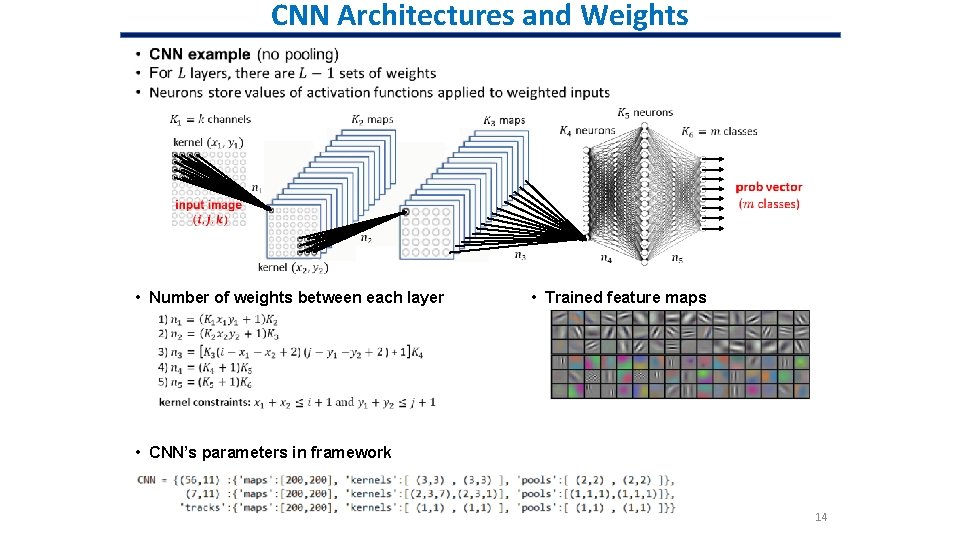
CNN Architectures and Weights • Number of weights between each layer • Trained feature maps • CNN’s parameters in framework 14

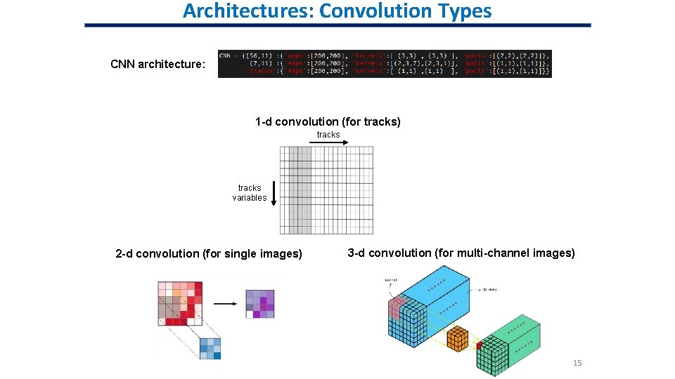
Architectures: Convolution Types CNN architecture: 1 -d convolution (for tracks) tracks variables 2 -d convolution (for single images) 3 -d convolution (for multi-channel images) 15

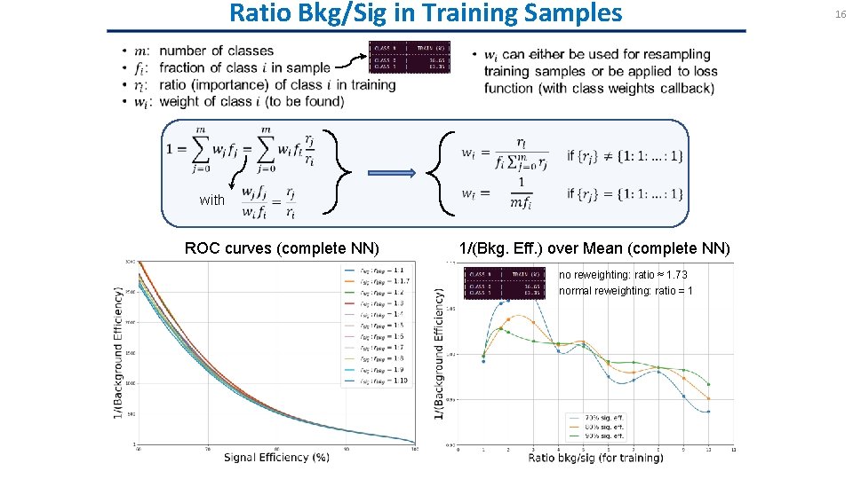
Ratio Bkg/Sig in Training Samples with ROC curves (complete NN) 1/(Bkg. Eff. ) over Mean (complete NN) no reweighting: ratio ≈ 1. 73 normal reweighting: ratio = 1 16

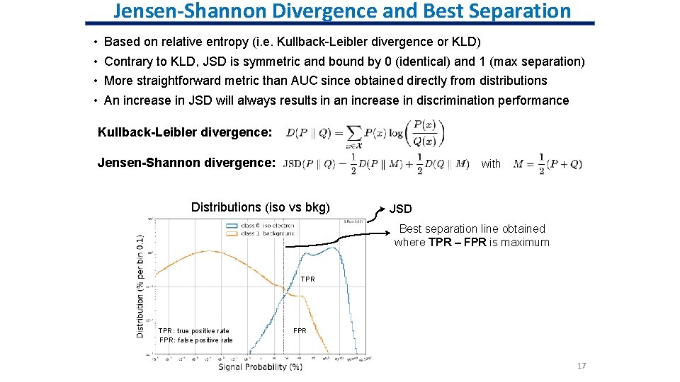
Jensen-Shannon Divergence and Best Separation • • Based on relative entropy (i. e. Kullback-Leibler divergence or KLD) Contrary to KLD, JSD is symmetric and bound by 0 (identical) and 1 (max separation) More straightforward metric than AUC since obtained directly from distributions An increase in JSD will always results in an increase in discrimination performance Kullback-Leibler divergence: Jensen-Shannon divergence: with Distributions (iso vs bkg) JSD Best separation line obtained where TPR – FPR is maximum TPR: true positive rate FPR: false positive rate FPR 17

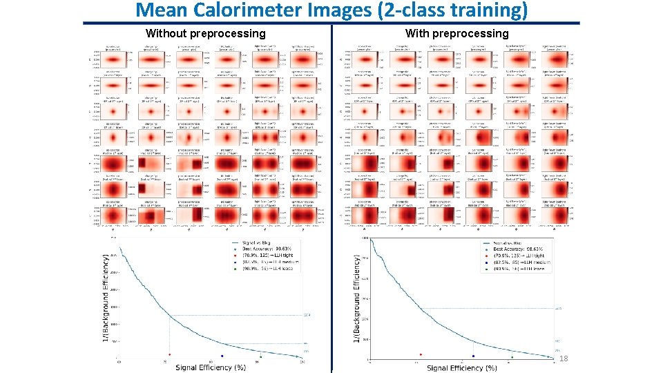
Mean Calorimeter Images (2 -class training) Without preprocessing With preprocessing 18

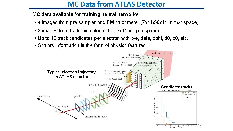
MC Data from ATLAS Detector MC data available for training neural networks • 4 images from pre-sampler and EM calorimeter (7 x 11/56 x 11 in ηxφ space) • 3 images from hadronic calorimeter (7 x 11 in ηxφ space) • Up to 10 track candidates per electron with p/e, deta, dphi, d 0, z 0, etc. • Scalars information in the form of physics features Typical electron trajectory in ATLAS detector Candidate tracks 19

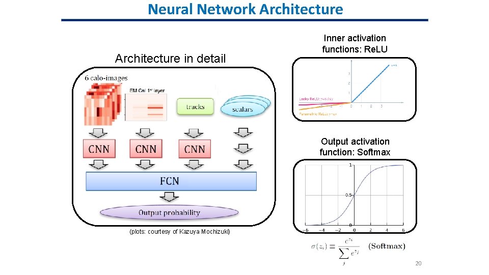
Neural Network Architecture in detail Inner activation functions: Re. LU Output activation function: Softmax (plots: courtesy of Kazuya Mochizuki) 20