EAT 213 FLUID MECHANICS AND HYDRAULICS WEEK 12

EAT 213 FLUID MECHANICS AND HYDRAULICS WEEK 12 -14 CHAPTER 14: OPEN CHANNEL FLOW SCHOOL OF ENVIRONMENTAL ENGINEERING UNIVERSITI MALAYSIA PERLIS 2017/2018

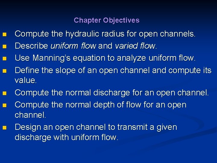
Chapter Objectives n n n n Compute the hydraulic radius for open channels. Describe uniform flow and varied flow. Use Manning’s equation to analyze uniform flow. Define the slope of an open channel and compute its value. Compute the normal discharge for an open channel. Compute the normal depth of flow for an open channel. Design an open channel to transmit a given discharge with uniform flow.

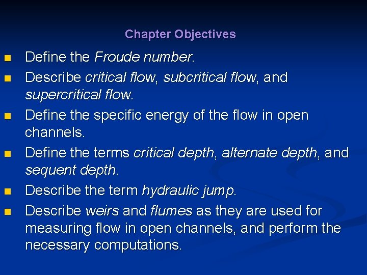
Chapter Objectives n n n Define the Froude number. Describe critical flow, subcritical flow, and supercritical flow. Define the specific energy of the flow in open channels. Define the terms critical depth, alternate depth, and sequent depth. Describe the term hydraulic jump. Describe weirs and flumes as they are used for measuring flow in open channels, and perform the necessary computations.

Chapter Outline 1. 2. 3. 4. 5. 6. 7. 8. 9. 10. Introductory Concepts Classification of Open-Channel Flow Hydraulic Radius and Reynolds Number in Open. Channel Flow Kinds of Open-Channel Flow Uniform Steady Flow in Open Channels The Geometry of Typical Open Channels The Most Efficient Shapes for Open Channels Critical Flow and Specific Energy Hydraulic Jump Open-Channel Flow Measurement

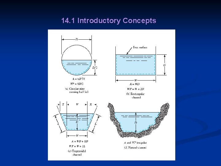
14. 1 Introductory Concepts n n Many examples of open channels occur in nature and in systems designed to supply water to communities or to carry storm drainage and sewage safely away. Fig 14. 1 shows the examples of cross sections of open channels.

14. 1 Introductory Concepts

14. 2 Classification of Open-Channel Flow n n Uniform steady flow occurs when the volume flow rate (typically called discharge in open-channel flow analysis) remains constant in the section of interest and the depth of the fluid in the channel does not vary. Figure 14. 2 shows uniform flow in a side view.

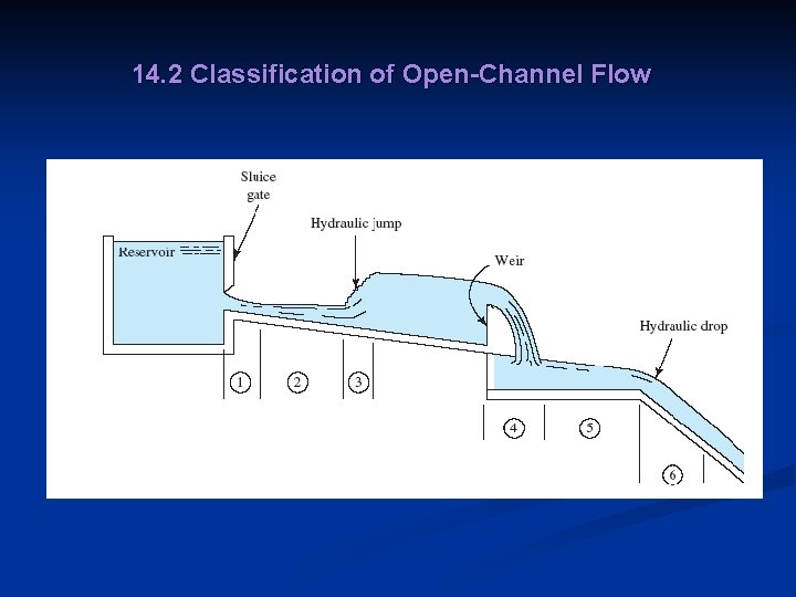
14. 2 Classification of Open-Channel Flow n n Varied steady flow occurs when the discharge remains constant but the depth of the fluid varies along the section of interest. Unsteady varied flow occurs when the discharge varies with time, resulting in changes in the depth of the fluid along the section of interest whether the channel is prismatic or not. Varied flow can be further classified into rapidly varying flow or gradually varying flow. Figure 14. 3 illustrates a series of conditions in which varied flow occurs.

14. 2 Classification of Open-Channel Flow

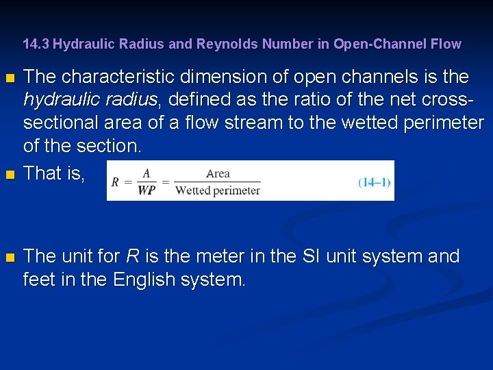
14. 3 Hydraulic Radius and Reynolds Number in Open-Channel Flow n n n The characteristic dimension of open channels is the hydraulic radius, defined as the ratio of the net crosssectional area of a flow stream to the wetted perimeter of the section. That is, The unit for R is the meter in the SI unit system and feet in the English system.

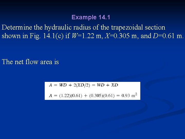
Example 14. 1 Determine the hydraulic radius of the trapezoidal section shown in Fig. 14. 1(c) if W=1. 22 m, X=0. 305 m, and D=0. 61 m. The net flow area is

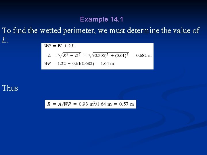
Example 14. 1 To find the wetted perimeter, we must determine the value of L: Thus

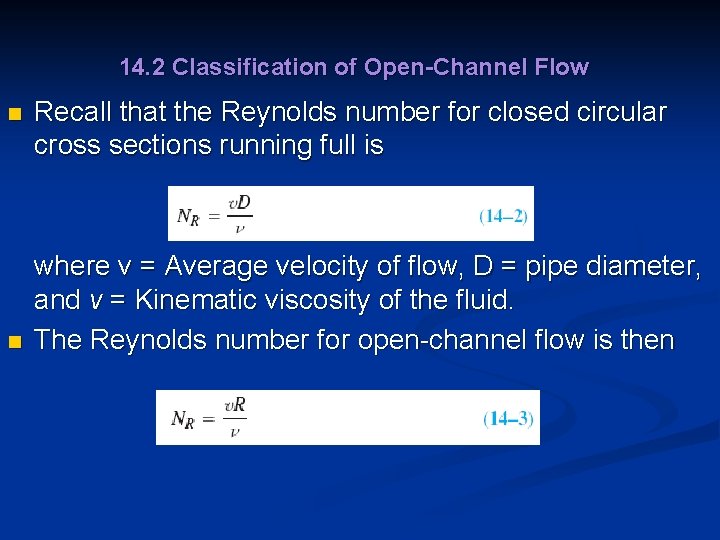
14. 2 Classification of Open-Channel Flow n n Recall that the Reynolds number for closed circular cross sections running full is where v = Average velocity of flow, D = pipe diameter, and v = Kinematic viscosity of the fluid. The Reynolds number for open-channel flow is then

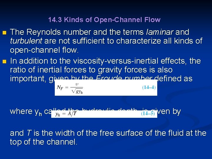
14. 3 Kinds of Open-Channel Flow n n The Reynolds number and the terms laminar and turbulent are not sufficient to characterize all kinds of open-channel flow. In addition to the viscosity-versus-inertial effects, the ratio of inertial forces to gravity forces is also important, given by the Froude number defined as where yh called the hydraulic depth, is given by and T is the width of the free surface of the fluid at the top of the channel.

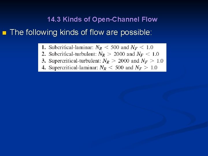
14. 3 Kinds of Open-Channel Flow n The following kinds of flow are possible:

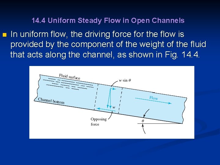
14. 4 Uniform Steady Flow in Open Channels n In uniform flow, the driving force for the flow is provided by the component of the weight of the fluid that acts along the channel, as shown in Fig. 14. 4.

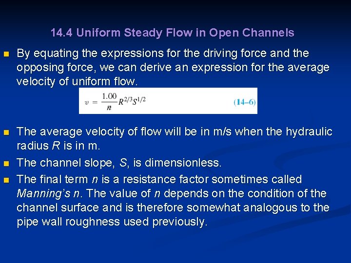
14. 4 Uniform Steady Flow in Open Channels n By equating the expressions for the driving force and the opposing force, we can derive an expression for the average velocity of uniform flow. n The average velocity of flow will be in m/s when the hydraulic radius R is in m. The channel slope, S, is dimensionless. The final term n is a resistance factor sometimes called Manning’s n. The value of n depends on the condition of the channel surface and is therefore somewhat analogous to the pipe wall roughness used previously. n n

14. 4 Uniform Steady Flow in Open Channels n Typical design values of n are listed in Table 14. 1 for materials commonly used for artificial channels and natural streams.

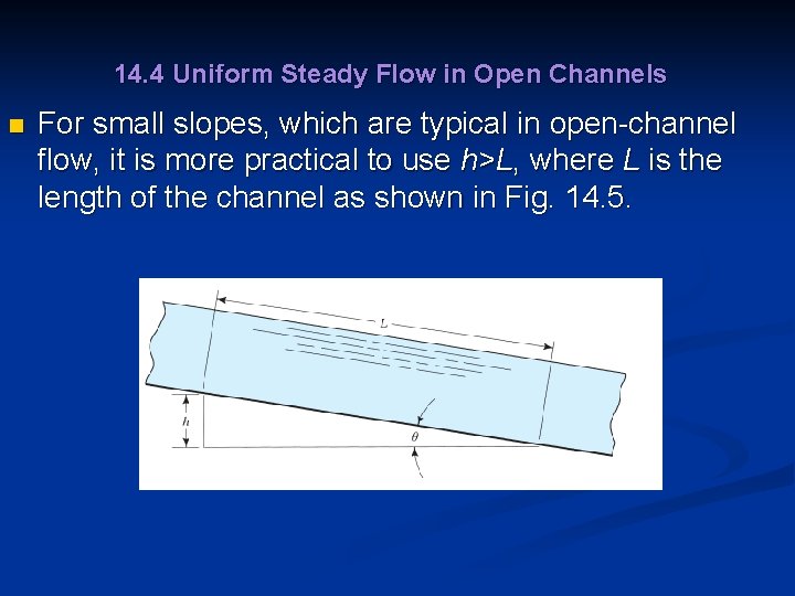
14. 4 Uniform Steady Flow in Open Channels n For small slopes, which are typical in open-channel flow, it is more practical to use h>L, where L is the length of the channel as shown in Fig. 14. 5.

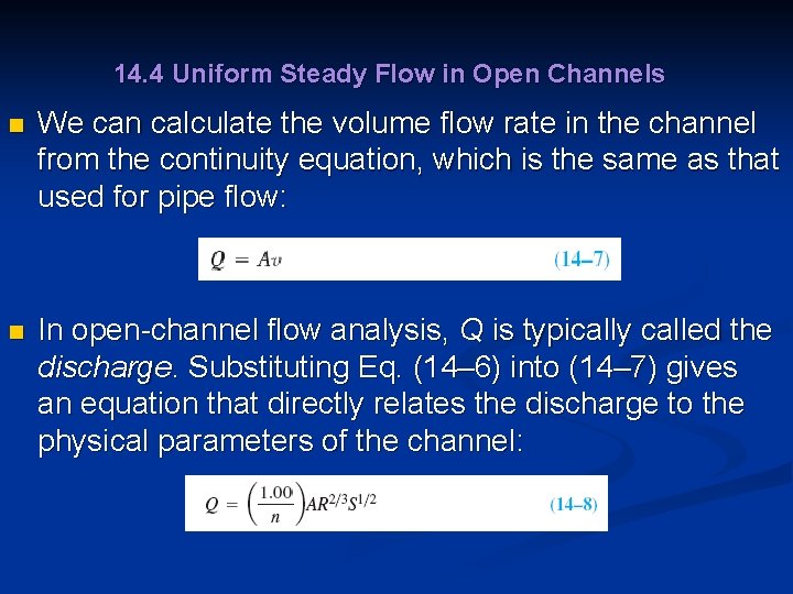
14. 4 Uniform Steady Flow in Open Channels n We can calculate the volume flow rate in the channel from the continuity equation, which is the same as that used for pipe flow: n In open-channel flow analysis, Q is typically called the discharge. Substituting Eq. (14– 6) into (14– 7) gives an equation that directly relates the discharge to the physical parameters of the channel:

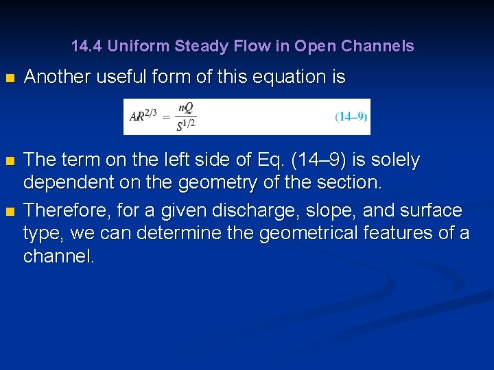
14. 4 Uniform Steady Flow in Open Channels n Another useful form of this equation is n The term on the left side of Eq. (14– 9) is solely dependent on the geometry of the section. Therefore, for a given discharge, slope, and surface type, we can determine the geometrical features of a channel. n

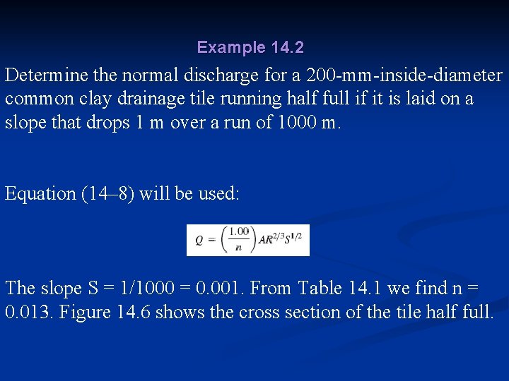
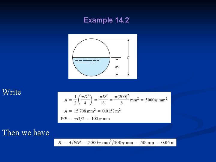
Example 14. 2 Determine the normal discharge for a 200 -mm-inside-diameter common clay drainage tile running half full if it is laid on a slope that drops 1 m over a run of 1000 m. Equation (14– 8) will be used: The slope S = 1/1000 = 0. 001. From Table 14. 1 we find n = 0. 013. Figure 14. 6 shows the cross section of the tile half full.

Example 14. 2 Write Then we have

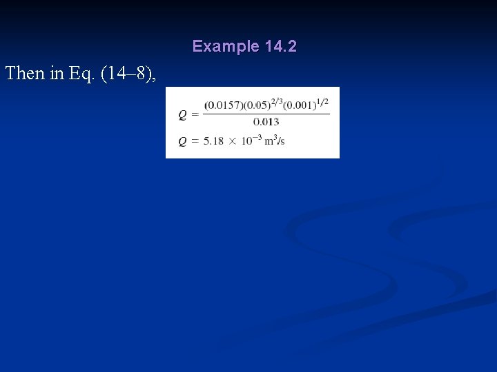
Example 14. 2 Then in Eq. (14– 8),

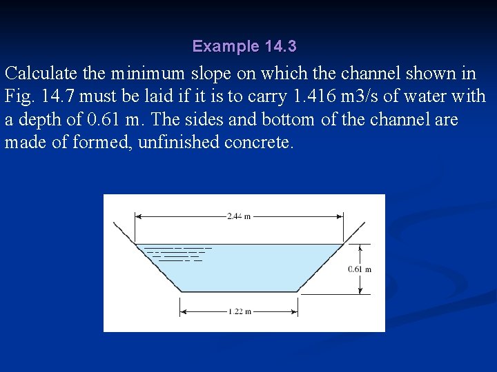
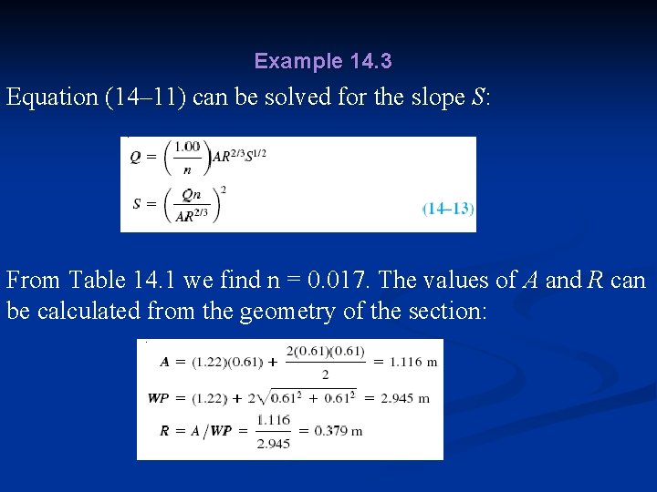
Example 14. 3 Calculate the minimum slope on which the channel shown in Fig. 14. 7 must be laid if it is to carry 1. 416 m 3/s of water with a depth of 0. 61 m. The sides and bottom of the channel are made of formed, unfinished concrete.

Example 14. 3 Equation (14– 11) can be solved for the slope S: From Table 14. 1 we find n = 0. 017. The values of A and R can be calculated from the geometry of the section:

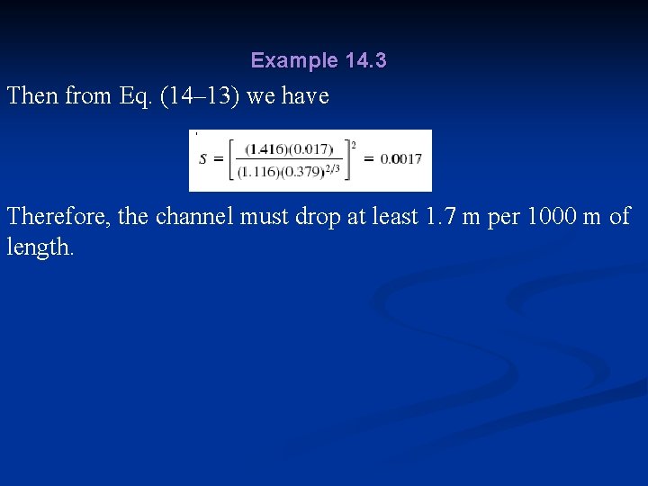
Example 14. 3 Then from Eq. (14– 13) we have Therefore, the channel must drop at least 1. 7 m per 1000 m of length.

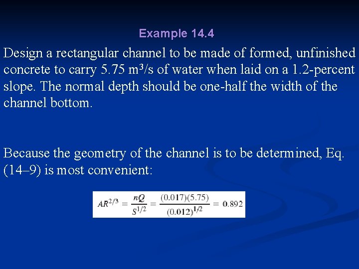
Example 14. 4 Design a rectangular channel to be made of formed, unfinished concrete to carry 5. 75 m 3/s of water when laid on a 1. 2 -percent slope. The normal depth should be one-half the width of the channel bottom. Because the geometry of the channel is to be determined, Eq. (14– 9) is most convenient:

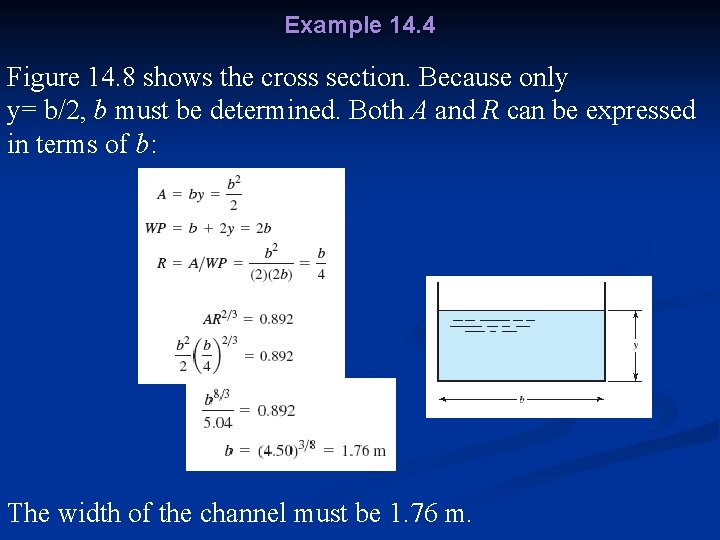
Example 14. 4 Figure 14. 8 shows the cross section. Because only y= b/2, b must be determined. Both A and R can be expressed in terms of b: The width of the channel must be 1. 76 m.

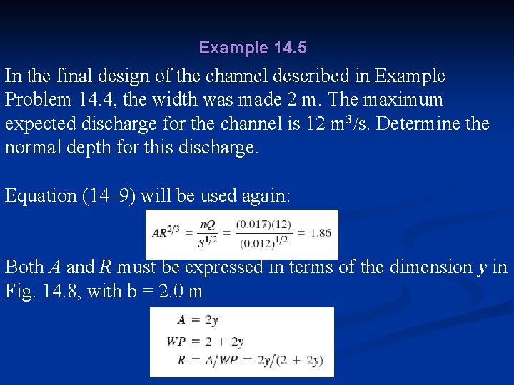
Example 14. 5 In the final design of the channel described in Example Problem 14. 4, the width was made 2 m. The maximum expected discharge for the channel is 12 m 3/s. Determine the normal depth for this discharge. Equation (14– 9) will be used again: Both A and R must be expressed in terms of the dimension y in Fig. 14. 8, with b = 2. 0 m

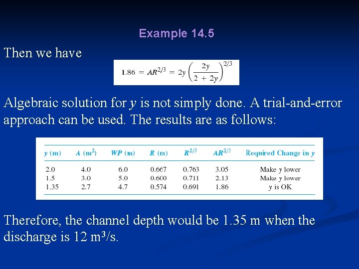
Example 14. 5 Then we have Algebraic solution for y is not simply done. A trial-and-error approach can be used. The results are as follows: Therefore, the channel depth would be 1. 35 m when the discharge is 12 m 3/s.

14. 6 The Geometry of Typical Open Channel n Table 14. 2 gives the formulas for computing the geometric features pertinent to open-channel flow calculations.

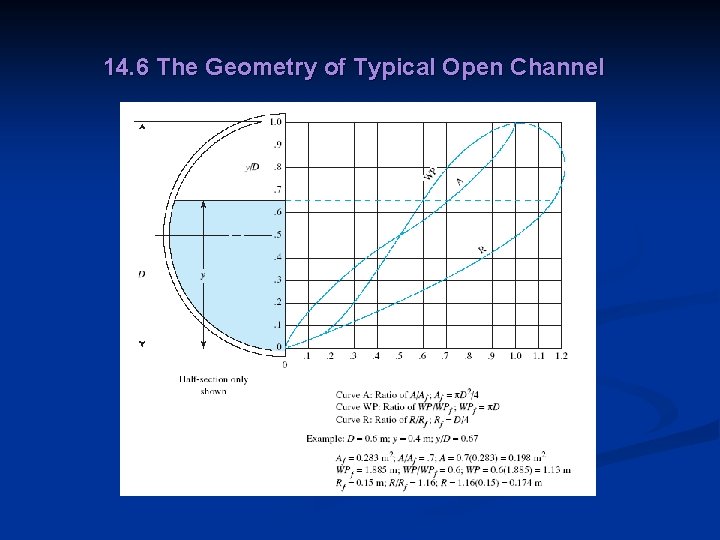
14. 6 The Geometry of Typical Open Channel n n The trapezoid is popular for several reasons. It is an efficient shape because it gives a large flow area relative to the wetted perimeter. The slope of the sides can be defined by the angle with respect to the horizontal or by means of the pitch, the ratio of the horizontal distance to the vertical distance. The computation of the data for circular sections at various depths can be facilitated by the graph in Fig. 14. 9.

14. 6 The Geometry of Typical Open Channel

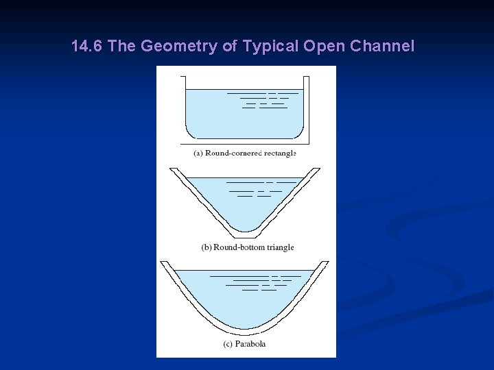
14. 6 The Geometry of Typical Open Channel n n Figure 14. 10 shows three other shapes used for open channels. Natural streams frequently can be approximated as shallow parabolas. The triangle with a rounded bottom is more practical to make in the earth than the sharp-V triangle. The round cornered rectangle performs somewhat better than the square-cornered rectangle and is easier to maintain.

14. 6 The Geometry of Typical Open Channel

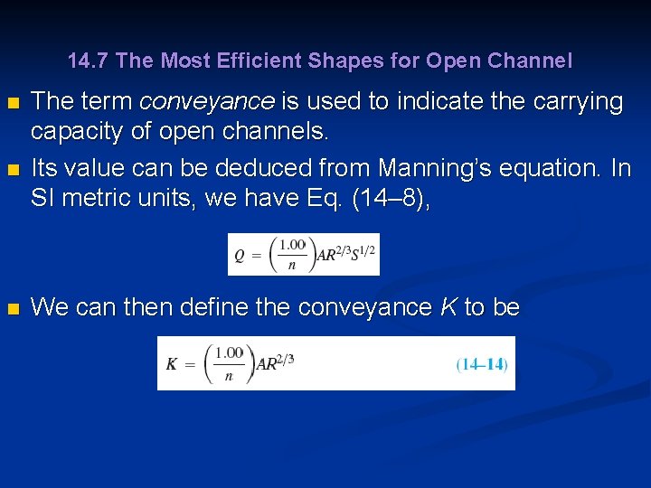
14. 7 The Most Efficient Shapes for Open Channel n n n The term conveyance is used to indicate the carrying capacity of open channels. Its value can be deduced from Manning’s equation. In SI metric units, we have Eq. (14– 8), We can then define the conveyance K to be

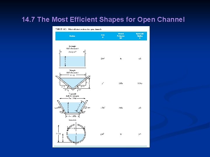
14. 7 The Most Efficient Shapes for Open Channel n In U. S. Customary units, n Manning’s equation is then n Table 14. 3 shows the most efficient designs of other shapes.

14. 7 The Most Efficient Shapes for Open Channel

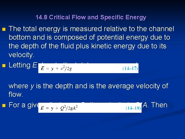
14. 8 Critical Flow and Specific Energy n The total energy is measured relative to the channel bottom and is composed of potential energy due to the depth of the fluid plus kinetic energy due to its velocity. Letting E denote the total energy, we get n where y is the depth and is the average velocity of flow. For a given discharge Q, the velocity is Q/A. Then n

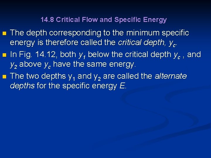
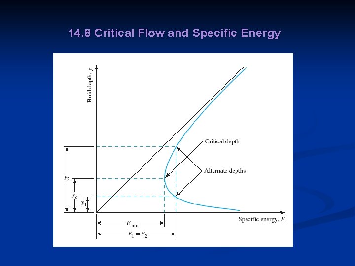
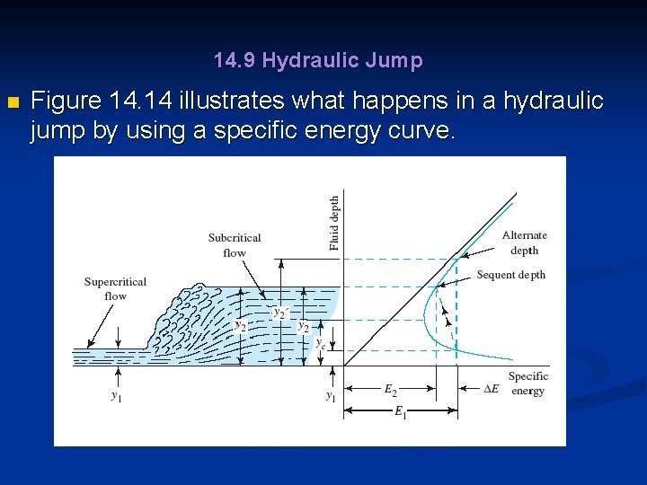
14. 8 Critical Flow and Specific Energy n n n The depth corresponding to the minimum specific energy is therefore called the critical depth, yc. In Fig. 14. 12, both y 1 below the critical depth yc , and y 2 above yc have the same energy. The two depths y 1 and y 2 are called the alternate depths for the specific energy E.

14. 8 Critical Flow and Specific Energy

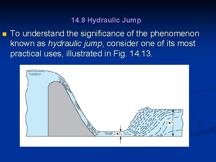
14. 9 Hydraulic Jump n To understand the significance of the phenomenon known as hydraulic jump, consider one of its most practical uses, illustrated in Fig. 14. 13.

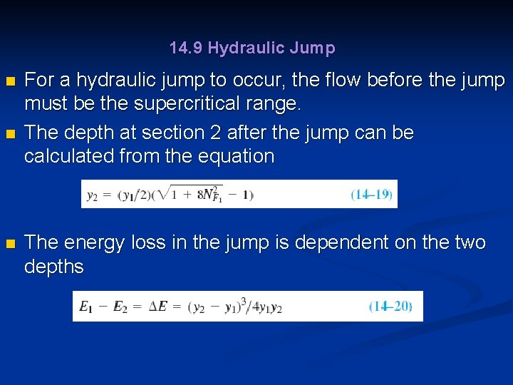
14. 9 Hydraulic Jump n n n For a hydraulic jump to occur, the flow before the jump must be the supercritical range. The depth at section 2 after the jump can be calculated from the equation The energy loss in the jump is dependent on the two depths

14. 9 Hydraulic Jump n Figure 14. 14 illustrates what happens in a hydraulic jump by using a specific energy curve.

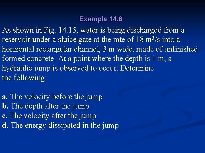
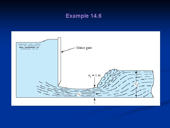
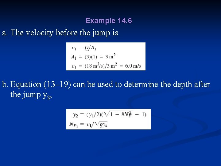
Example 14. 6 As shown in Fig. 14. 15, water is being discharged from a reservoir under a sluice gate at the rate of 18 m 3/s into a horizontal rectangular channel, 3 m wide, made of unfinished formed concrete. At a point where the depth is 1 m, a hydraulic jump is observed to occur. Determine the following: a. The velocity before the jump b. The depth after the jump c. The velocity after the jump d. The energy dissipated in the jump

Example 14. 6

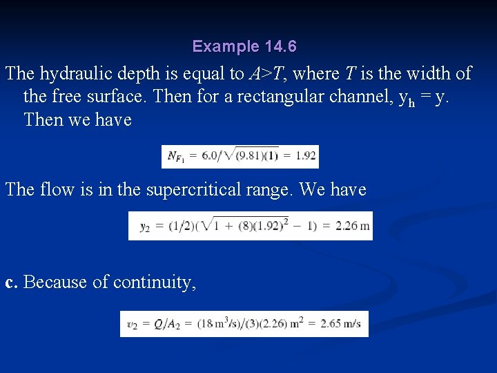
Example 14. 6 a. The velocity before the jump is b. Equation (13– 19) can be used to determine the depth after the jump y 2,

Example 14. 6 The hydraulic depth is equal to A>T, where T is the width of the free surface. Then for a rectangular channel, yh = y. Then we have The flow is in the supercritical range. We have c. Because of continuity,

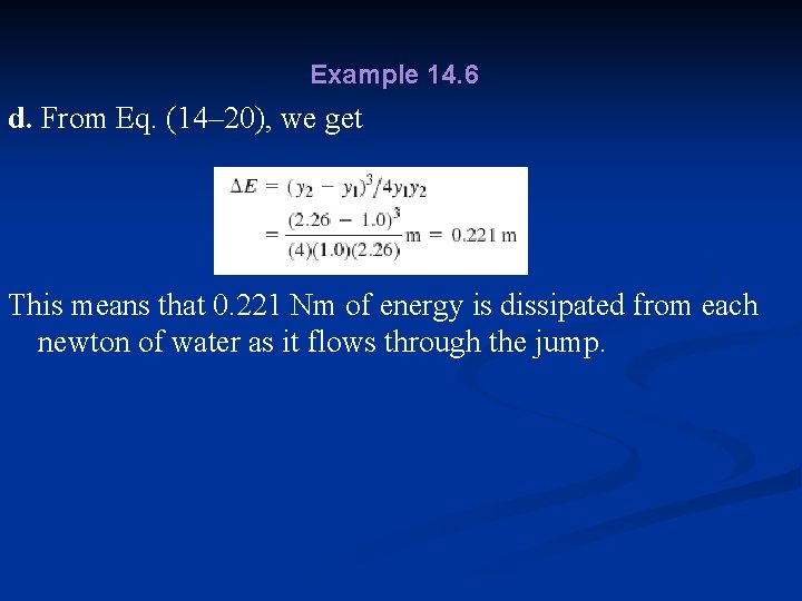
Example 14. 6 d. From Eq. (14– 20), we get This means that 0. 221 Nm of energy is dissipated from each newton of water as it flows through the jump.

14. 10 Open-Channel Flow Measurement n n An open channel is one that has its top surface open to the prevailing atmosphere. Two widely used devices for open-channel flow measurement are weirs and flumes. Each causes the area of the stream to change, which in turn changes the level of the fluid surface. The resulting level of the surface relative to some feature of the device is related to the quantity of flow.

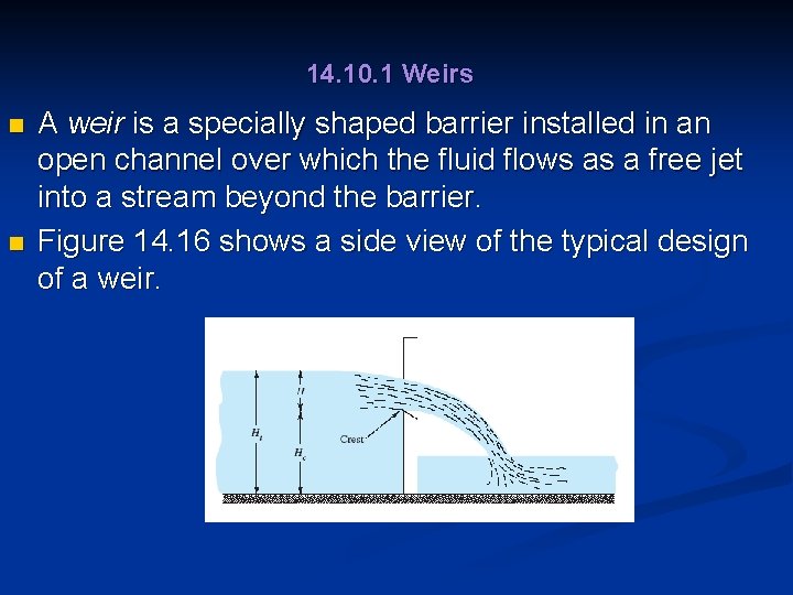
14. 10. 1 Weirs n n A weir is a specially shaped barrier installed in an open channel over which the fluid flows as a free jet into a stream beyond the barrier. Figure 14. 16 shows a side view of the typical design of a weir.

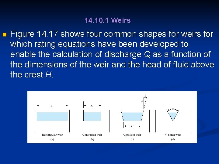
14. 10. 1 Weirs n Figure 14. 17 shows four common shapes for weirs for which rating equations have been developed to enable the calculation of discharge Q as a function of the dimensions of the weir and the head of fluid above the crest H.

14. 10. 1 Weirs n n Measurement of the head can be by a fixed gage, called a staff gage, mounted at the side of the stream for which the zero reading is at the level of the crest of the weir. A rectangular weir, also called a suppressed weir, has a crest length L that extends the full width of the channel into which it is installed.

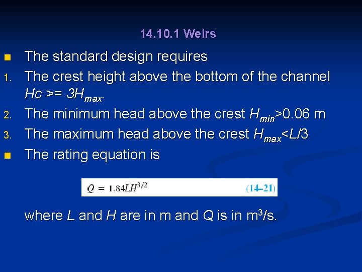
14. 10. 1 Weirs n 1. 2. 3. n The standard design requires The crest height above the bottom of the channel Hc >= 3 Hmax. The minimum head above the crest Hmin>0. 06 m The maximum head above the crest Hmax<L/3 The rating equation is where L and H are in m and Q is in m 3/s.

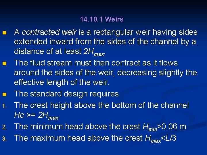
14. 10. 1 Weirs n n n 1. 2. 3. A contracted weir is a rectangular weir having sides extended inward from the sides of the channel by a distance of at least 2 Hmax. The fluid stream must then contract as it flows around the sides of the weir, decreasing slightly the effective length of the weir. The standard design requires The crest height above the bottom of the channel Hc >= 2 Hmax. The minimum head above the crest Hmin>0. 06 m The maximum head above the crest Hmax<L/3

14. 10. 1 Weirs n n n The rating equation is where L and H are in m and Q is in m 3/s. A Cipolletti weir is also contracted from the sides of the stream by a distance at least 2 Hmax and has sides that are sloped outward as shown in Fig. 14. 17(c). The same requirements listed for the contracted rectangular weir apply. The rating equation is

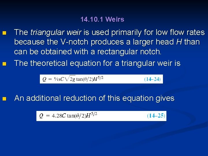
14. 10. 1 Weirs n The triangular weir is used primarily for low flow rates because the V-notch produces a larger head H than can be obtained with a rectangular notch. The theoretical equation for a triangular weir is n An additional reduction of this equation gives n

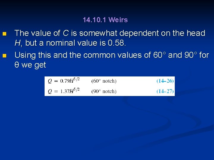
14. 10. 1 Weirs n n The value of C is somewhat dependent on the head H, but a nominal value is 0. 58. Using this and the common values of 60° and 90° for θ we get

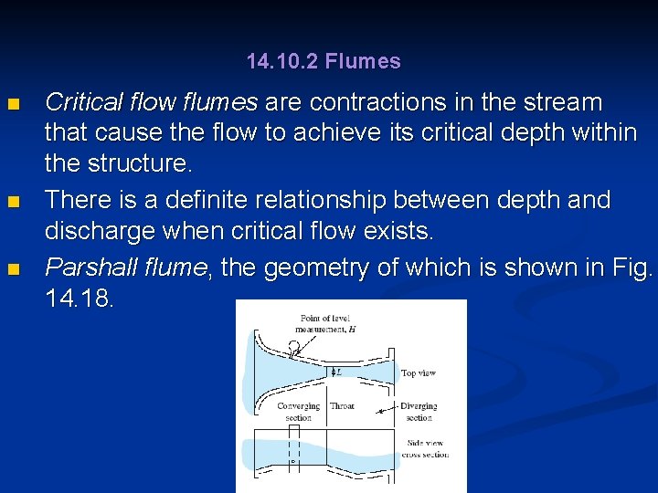
14. 10. 2 Flumes n n n Critical flow flumes are contractions in the stream that cause the flow to achieve its critical depth within the structure. There is a definite relationship between depth and discharge when critical flow exists. Parshall flume, the geometry of which is shown in Fig. 14. 18.

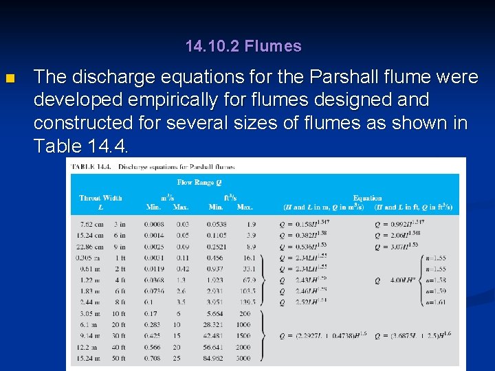
14. 10. 2 Flumes n The discharge equations for the Parshall flume were developed empirically for flumes designed and constructed for several sizes of flumes as shown in Table 14. 4.

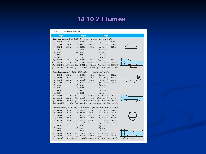
14. 10. 2 Flumes n n Long-throated flumes, rather than Parshall flumes, are recommended for new construction because they are simpler and less expensive to build and can more easily be adapted to channels with a variety of shapes. Table 14. 5 shows the general shape consisting of a straight ramp up from the bottom of the channel, a flat throat section, and a sudden drop.

14. 10. 2 Flumes

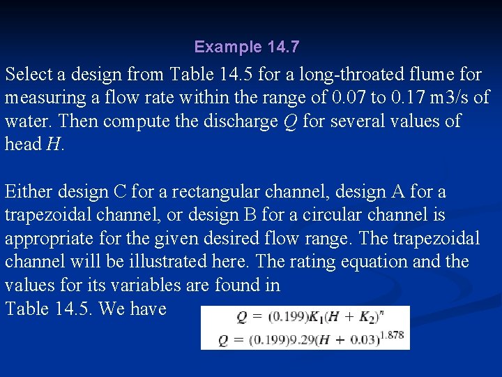
Example 14. 7 Select a design from Table 14. 5 for a long-throated flume for measuring a flow rate within the range of 0. 07 to 0. 17 m 3/s of water. Then compute the discharge Q for several values of head H. Either design C for a rectangular channel, design A for a trapezoidal channel, or design B for a circular channel is appropriate for the given desired flow range. The trapezoidal channel will be illustrated here. The rating equation and the values for its variables are found in Table 14. 5. We have

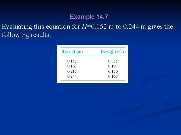
Example 14. 7 Evaluating this equation for H=0. 152 m to 0. 244 m gives the following results:

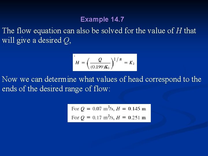
Example 14. 7 The flow equation can also be solved for the value of H that will give a desired Q, Now we can determine what values of head correspond to the ends of the desired range of flow: