Dynamical Forecasting Dr Mark Cresswell 69 EG 6517

Dynamical Forecasting Dr Mark Cresswell 69 EG 6517 – Impacts & Models of Climate Change

Lecture Topics • What is dynamical forecasting? • • • Equations used Operational procedures Ensemble forecasting The “bin” approach (terciles and quintiles) Estimation of accuracy and skill Case Study – West Africa

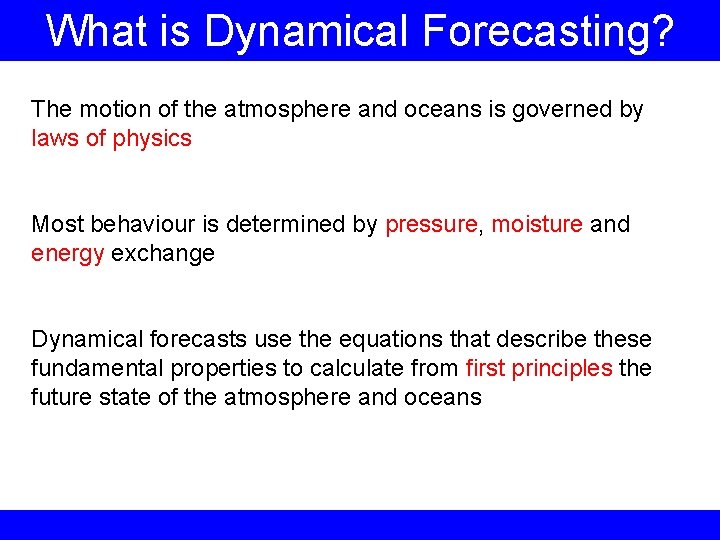
What is Dynamical Forecasting? The motion of the atmosphere and oceans is governed by laws of physics Most behaviour is determined by pressure, moisture and energy exchange Dynamical forecasts use the equations that describe these fundamental properties to calculate from first principles the future state of the atmosphere and oceans

What is Dynamical Forecasting? Dynamical forecasts are not reliant upon a knowledge of past climatic events as statistical forecasts are Dynamical forecasts may suggest large anomalous shifts in climate as a result of their physics – an advantage if such a signal is real or potentially a serious flaw if the signal is merely transient Dynamical forecasts are only as good as the data they are initialised with and the physics/parameterisation schemes they employ to calculate pressure, humidity and energy flux

Equations Used The equations used in a climate model are not particularly difficult to solve It is the number of equations that must be solved for each time-step for a single integration that is a burden Fundamental equations may have to be altered in order to be more representative of a particular process. Vertical exchanges (involving height) are adiabatic and more complex Essentially the equations describe a fluid and entropy

Equations Used The FIRST law of thermodynamics describes how the state of a system changes in response to work it performs and heat absorbed by it The SECOND law of thermodynamics deals with the direction of thermodynamic processes and the efficiency with which they occur. Since these characteristics control how a system evolves out of a given state, the second law also underlies the stability of thermodynamic equilibrium

Operational procedures The following steps are used to generate a single forecast: 1. Assimilation of observations 2. Calculation of all starting state variables 3. Time-step uses sets of differential equations 4. New values of state variables become starting conditions 5. Further time-steps project beyond spin-up period 6. Once state has evolved to desired time model is stopped 7. Values of state variables (forecast fields) extracted

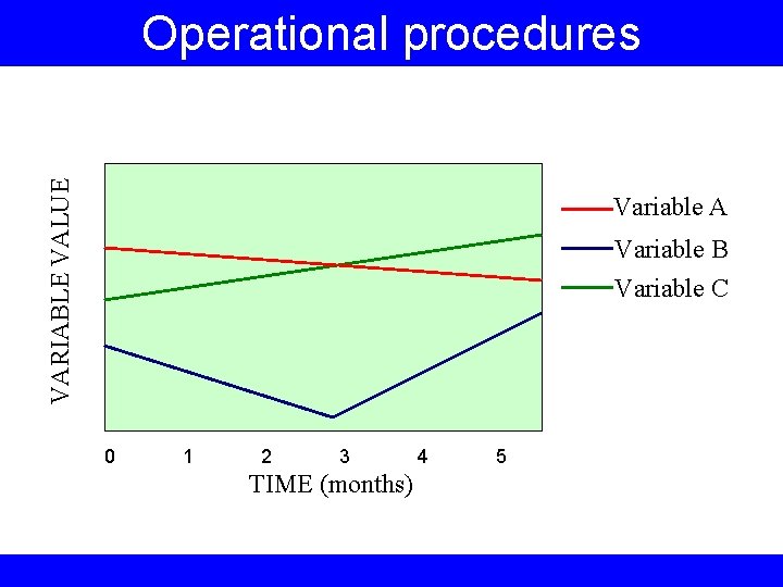
VARIABLE VALUE Operational procedures Variable A Variable B Variable C 0 1 2 3 TIME (months) 4 5

Operational procedures • The problem with running a single model integration is that it is effectively a deterministic solution – values of variables have only a single outcome • It is desirable to sample the uncertainty of the future state as much as possible and hopefully extract as much predictability (and hence signal) as the system allows • Once way to do this is to use an ensemble prediction system (EPS). This approach maximises any causal predictability (increases signal: noise ratio) and allows probability estimates to be generated

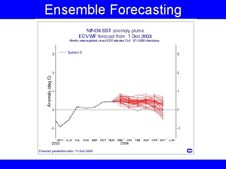
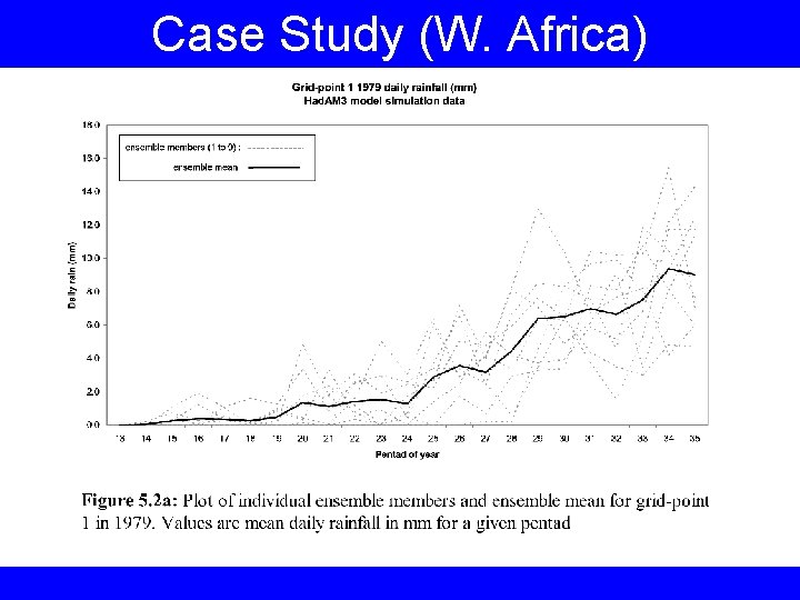
Ensemble Forecasting • An ensemble is merely a collection of individual forecast integrations – called members • Each member is produced from a forecast run initialised one day apart from the next • If there is any predictability (a strong SST anomaly for example) most of the members should remain close together through time • Poor predictability is characterised by members diverging from each other early on • Taking the average of all members for any given time (the ensemble-mean) is a monte-carlo simulation

Ensemble Forecasting

Ensemble Forecasting The greater the number of ensemble members, the greater is the clarity of the forcing signal which determines the future state of the atmosphere Large ensembles also sample more of the uncertainty and hence provide a more significant forecast than fewer members might give Ensemble prediction systems allow the generation of probabilistic forecasts using categorical “bin” approaches

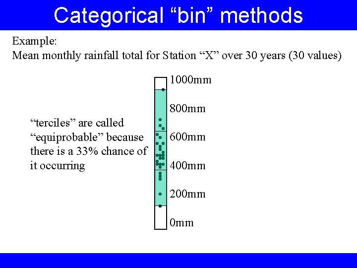
Categorical “bin” methods A new and very powerful way of creating probabilistic forecasts is based on categorical analysis Analysis of historical data (climatologies of about 30 years) provides us with a knowledge of the frequency of specific climate states We can build up a statistical picture of how variable (extreme) climate states can be – and hence what constitutes “normal” conditions

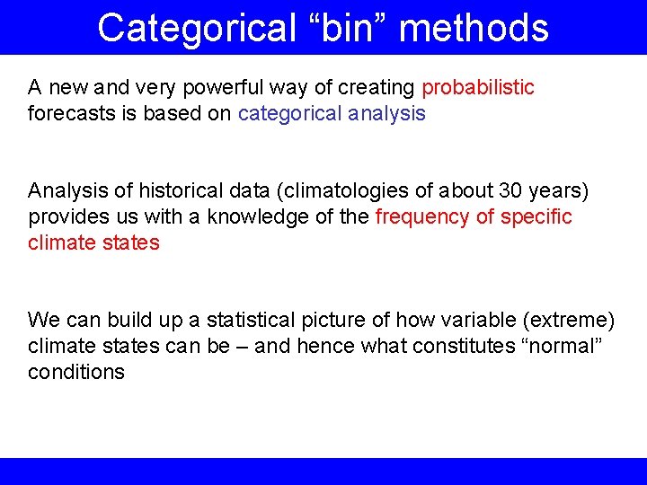
Categorical “bin” methods Example: Mean monthly rainfall total for Station “X” over 30 years (30 values) • 1000 mm 800 mm • • • 600 mm • • • • 400 mm • • • • 200 mm • 0 mm

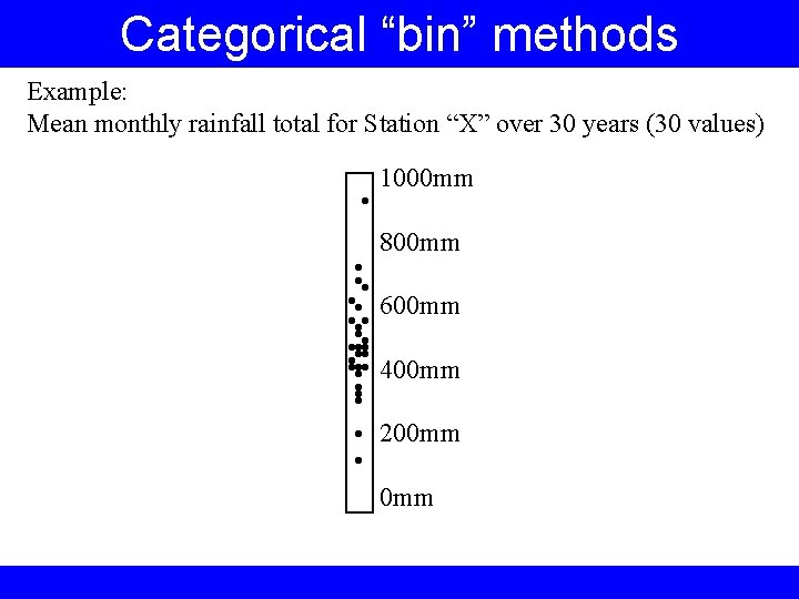
Categorical “bin” methods Example: Mean monthly rainfall total for Station “X” over 30 years (30 values) • 1000 mm 800 mm range • • • 600 mm • • • • 400 mm • • • • 200 mm • 0 mm

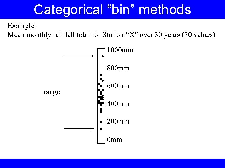
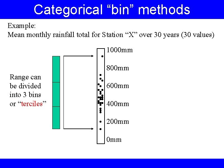
Categorical “bin” methods Example: Mean monthly rainfall total for Station “X” over 30 years (30 values) • 1000 mm 800 mm Range can be divided into 3 bins or “terciles” • • • 600 mm • • • • 400 mm • • • • 200 mm • 0 mm

Categorical “bin” methods Example: Mean monthly rainfall total for Station “X” over 30 years (30 values) • 1000 mm 800 mm “terciles” are called “equiprobable” because there is a 33% chance of it occurring • • • 600 mm • • • • 400 mm • • • • 200 mm • 0 mm

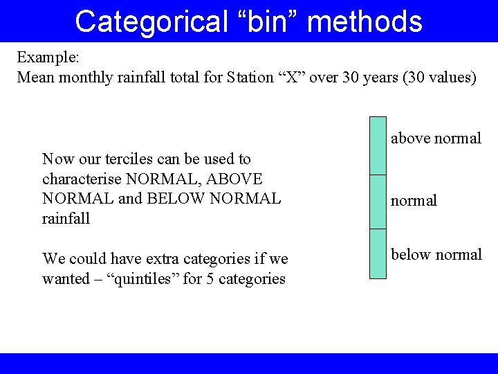
Categorical “bin” methods Example: Mean monthly rainfall total for Station “X” over 30 years (30 values) above normal Now our terciles can be used to characterise NORMAL, ABOVE NORMAL and BELOW NORMAL rainfall We could have extra categories if we wanted – “quintiles” for 5 categories normal below normal

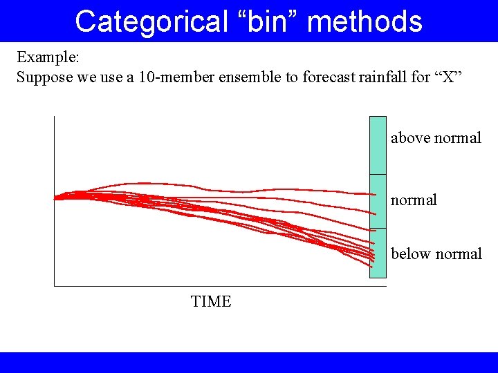
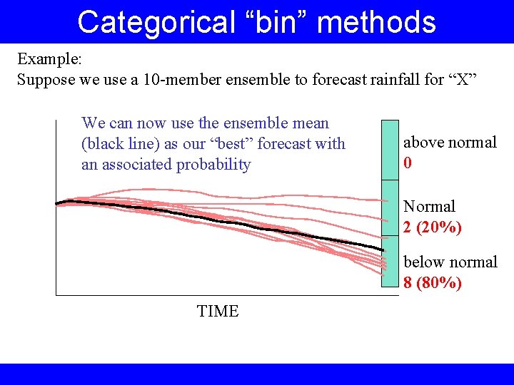
Categorical “bin” methods Example: Suppose we use a 10 -member ensemble to forecast rainfall for “X” above normal below normal TIME

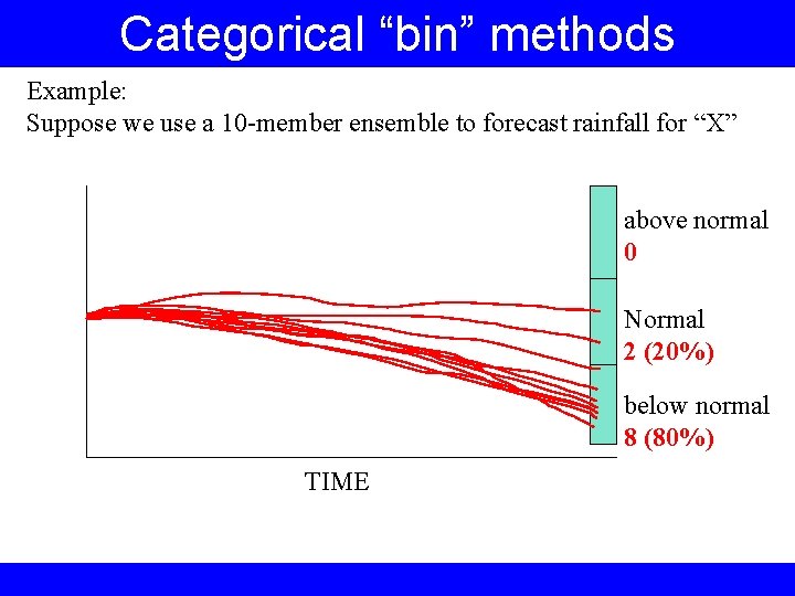
Categorical “bin” methods Example: Suppose we use a 10 -member ensemble to forecast rainfall for “X” above normal 0 Normal 2 (20%) below normal 8 (80%) TIME

Categorical “bin” methods Example: Suppose we use a 10 -member ensemble to forecast rainfall for “X” We can now use the ensemble mean (black line) as our “best” forecast with an associated probability above normal 0 Normal 2 (20%) below normal 8 (80%) TIME

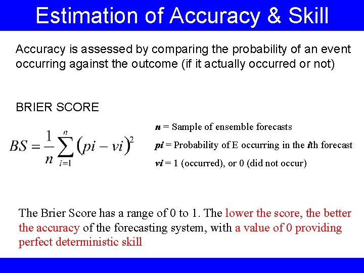
Estimation of Accuracy & Skill Accuracy is assessed by comparing the probability of an event occurring against the outcome (if it actually occurred or not) BRIER SCORE n = Sample of ensemble forecasts pi = Probability of E occurring in the ith forecast vi = 1 (occurred), or 0 (did not occur) The Brier Score has a range of 0 to 1. The lower the score, the better the accuracy of the forecasting system, with a value of 0 providing perfect deterministic skill

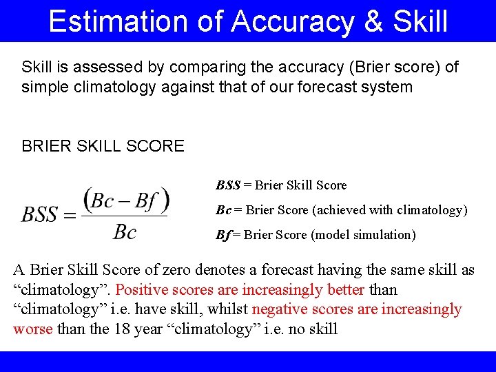
Estimation of Accuracy & Skill is assessed by comparing the accuracy (Brier score) of simple climatology against that of our forecast system BRIER SKILL SCORE BSS = Brier Skill Score Bc = Brier Score (achieved with climatology) Bf = Brier Score (model simulation) A Brier Skill Score of zero denotes a forecast having the same skill as “climatology”. Positive scores are increasingly better than “climatology” i. e. have skill, whilst negative scores are increasingly worse than the 18 year “climatology” i. e. no skill

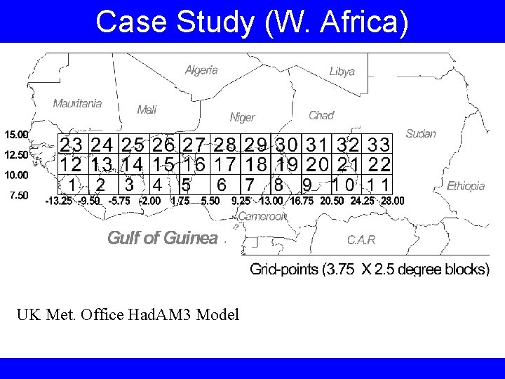
Case Study (W. Africa) UK Met. Office Had. AM 3 Model

Case Study (W. Africa)

Case Study (W. Africa)

Case Study (W. Africa)

Case Study (W. Africa)

Case Study (W. Africa)