DR Gatot F Hertono MSc Design and Analysis

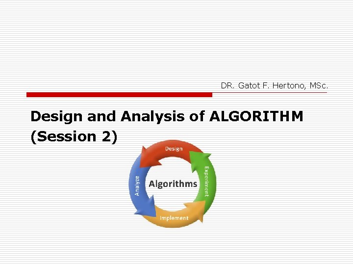
DR. Gatot F. Hertono, MSc. Design and Analysis of ALGORITHM (Session 2)

Our Machine Model: Assumptions Generic Random Access Machine (RAM) o Executes operations sequentially o Set of basic operations: n Arithmetic. Logical, Comparisons, Function calls o Simplifying assumption: all ops cost 1 unit Notes: n Eliminates dependence on the speed of our computer, otherwise impossible to verify and to compare

Running time • The running time depends on the input. Example: an already sorted sequence is easier to sort. • Major Simplifying Convention: Parameterize the running time by the size of the input. ØTA(n) = time of A on length n inputs • Generally, we seek upper bounds on the running time, to have a guarantee of performance.

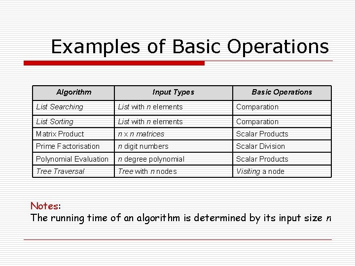
Examples of Basic Operations Algorithm Input Types Basic Operations List Searching List with n elements Comparation List Sorting List with n elements Comparation Matrix Product n x n matrices Scalar Products Prime Factorisation n digit numbers Scalar Division Polynomial Evaluation n degree polynomial Scalar Products Tree Traversal Tree with n nodes Visiting a node Notes: The running time of an algorithm is determined by its input size n

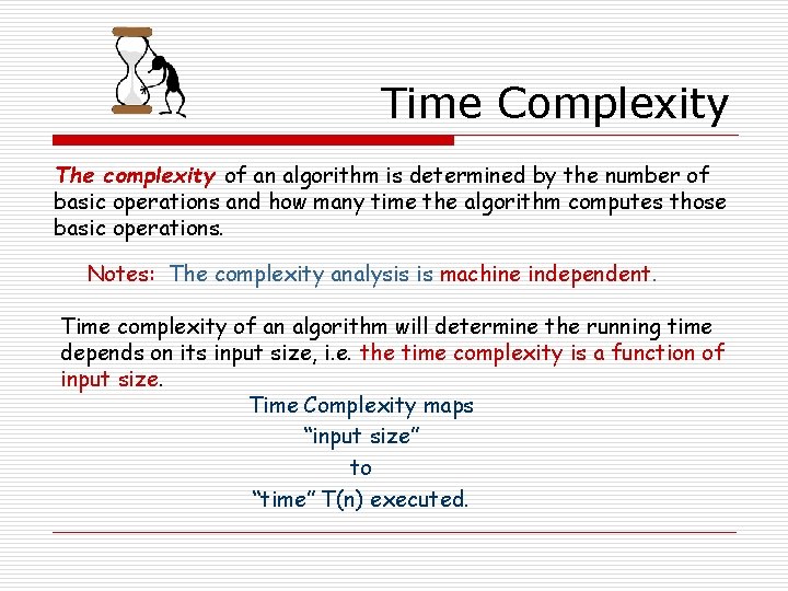
Time Complexity The complexity of an algorithm is determined by the number of basic operations and how many time the algorithm computes those basic operations. Notes: The complexity analysis is machine independent. Time complexity of an algorithm will determine the running time depends on its input size, i. e. the time complexity is a function of input size. Time Complexity maps “input size” to “time” T(n) executed.

Purpose o To estimate how long a program will run. o To estimate the largest input that can reasonably be given to the program. o To compare the efficiency of different algorithms. o To help focus on the parts of code that are executed the largest number of times. o To choose an algorithm for an application.

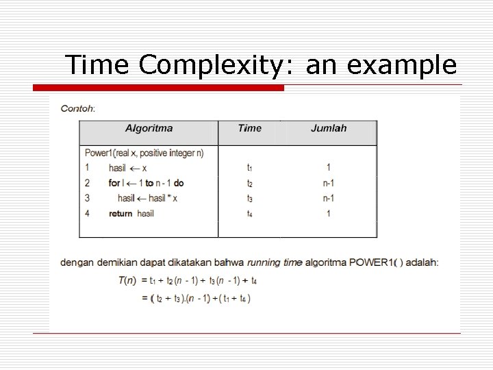
Time Complexity: an example

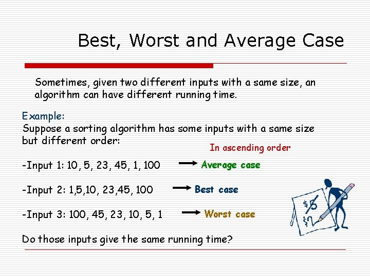
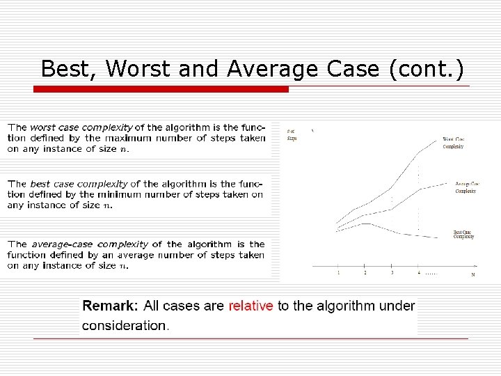
Best, Worst and Average Case Sometimes, given two different inputs with a same size, an algorithm can have different running time. Example: Suppose a sorting algorithm has some inputs with a same size but different order: In ascending order -Input 1: 10, 5, 23, 45, 1, 100 -Input 2: 1, 5, 10, 23, 45, 100 -Input 3: 100, 45, 23, 10, 5, 1 Average case Best case Worst case Do those inputs give the same running time?

Best, Worst and Average Case (cont. )

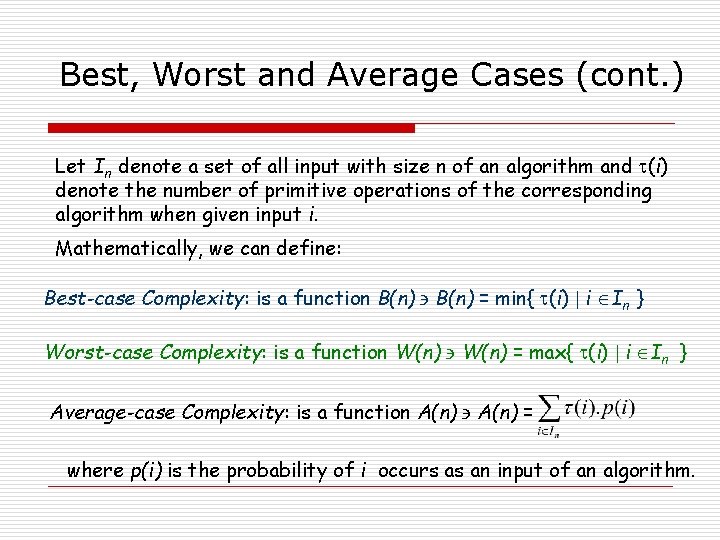
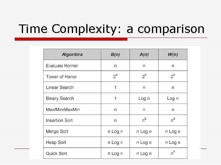
Best, Worst and Average Cases (cont. ) Let In denote a set of all input with size n of an algorithm and (i) denote the number of primitive operations of the corresponding algorithm when given input i. Mathematically, we can define: Best-case Complexity: is a function B(n) = min{ (i) i In } Worst-case Complexity: is a function W(n) = max{ (i) i In } Average-case Complexity: is a function A(n) = where p(i) is the probability of i occurs as an input of an algorithm.

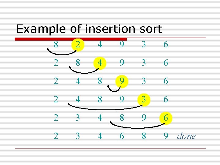
Example of insertion sort 8 2 4 9 3 6 2 8 4 9 3 6 2 4 8 9 3 6 2 3 4 8 9 6 2 3 4 6 8 9 done

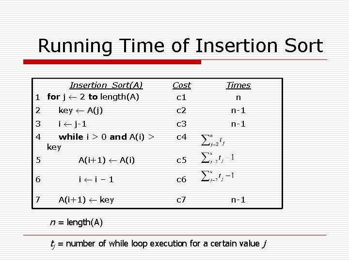
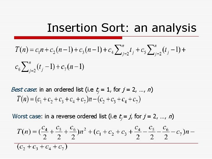
Running Time of Insertion Sort Insertion_Sort(A) 1 for j 2 to length(A) Cost c 1 Times n 2 key A(j) c 2 n-1 3 i j-1 c 3 n-1 4 while i > 0 and A(i) > key c 4 5 A(i+1) A(i) c 5 6 i i– 1 c 6 7 A(i+1) key c 7 n-1 n = length(A) tj = number of while loop execution for a certain value j

Insertion Sort: an analysis Best case: in an ordered list (i. e tj = 1, for j = 2, …, n) Worst case: in a reverse ordered list (i. e tj = j, for j = 2, …, n)

Time Complexity: a comparison

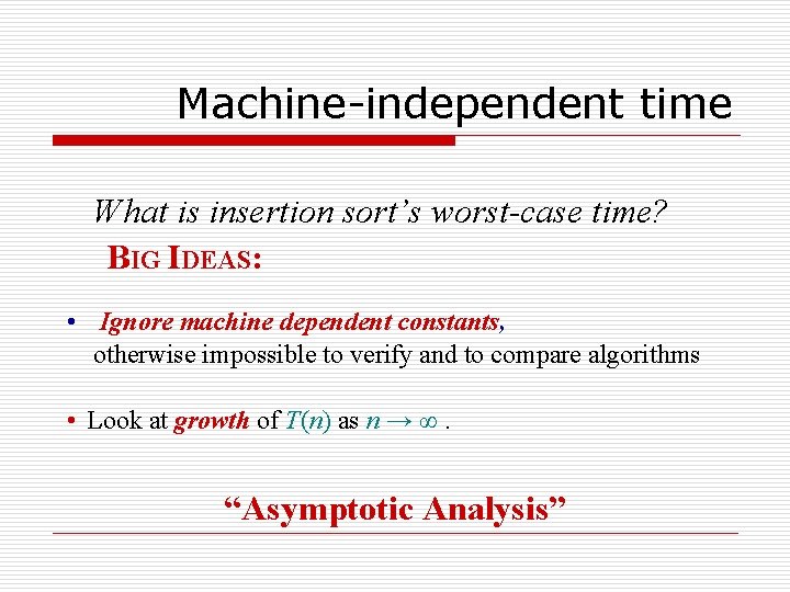
Machine-independent time What is insertion sort’s worst-case time? BIG IDEAS: • Ignore machine dependent constants, otherwise impossible to verify and to compare algorithms • Look at growth of T(n) as n → ∞. “Asymptotic Analysis”

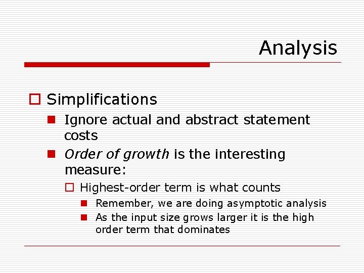
Analysis o Simplifications n Ignore actual and abstract statement costs n Order of growth is the interesting measure: o Highest-order term is what counts n Remember, we are doing asymptotic analysis n As the input size grows larger it is the high order term that dominates

Assignment 1 o In order to show that an algorithm is not unique, design two different algorithms of a specific problem. o Design an algorithm and show its time complexity to compute a product of two n x n matrices (how is the time complexity in the best and worst cases? )

Performance & Speed