Deep Belief Nets II Tai Sing Lee 15

Deep Belief Nets II Tai Sing Lee 15 -381/681 AI Lecture 13 Supplementary readings: Hinton, G. E. (2007) Learning multiple layers of representations, recommended. See other papers for optional reading. With thanks Geoff Hinton for slides in this DBN lecture, and G. A. Di Caro for the conditional independence slides.

Mid-term preparation • For my part: Study the pool questions during class, focused on basic concepts, maybe do some simple calculations. • Probability. Remember chain rule, Bayes rule, sum rule. • Bayes Net – conditional independence, chain rule, factorization. • Sampling – understand the different sampling methods and the motivation and situations for using them. • Deep belief net -- BM and r. BM, deep r. BM, basic concepts, what they can do. • Focus on concepts, rather than memorization of equations

Independence & information propagation • Question: Given a BN structure what dependence and independence relationships are represented? • How information propagates over the network? 3

Independence & information propagation Types of probabilistic relationships 4
 • If neither Z nor any of its descendants are")
Converging connection (common effect) • If neither Z nor any of its descendants are observed, X and Y are independent. • Information cannot be transmitted through Z among parents of Z. • If Z or any of its descendants are observed, X and Y are dependent. • Information can be transmitted through Z among parents of Z if Z or any of its descendants are observed. Observing Z or its descendants opens the information path. 5

Pool : Are C and D independent, given { X}? 1. 2. 3. 4. 5. False. True, False, True, True False, True, False, True, False, True 6

Markov Chain Monte Carlo Methods • Direct, rejection and likelihood weighting methods generate each new sample from scratch • MCMC generate each new sample by making a random change to preceding sample 7

Belief Nets • A belief net is a directed acyclic graph composed of stochastic variables. • Hidden variables (not observed) and visible variables • The inference problem: Infer the states of the unobserved variables. • The learning problem: Learn interaction between variables to make the network more likely to generate the observed data. stochastic hidden causes visible units: observations
 Energy of a state Probability of being")
The Boltzmann Machine (Hinton and Sejnowski 1985) Energy of a state Probability of being in a state T=w connections

Pool • Which of the following three sampled configurations of states has the higher probability of occurring? 1 0. 8 0. 9 A 1 2 3 4 -1 0. 8 1 0. 2 1 -0. 7 -1 1 0. 9 0. 8 -1 0. 2 -1 B A B C Not sure. 0. 9 1 -0. 7 0. 2 -1 C -1 -0. 7 -1

Learning in Boltzmann machine Hebbian learning fantasy/expectation input Direct sampling from the distributions Learn to model the data distribution of the observable units.
 • We restrict the connectivity")
Restricted Boltzmann Machines (Smolensky , 1986, called them “harmoniums”) • We restrict the connectivity to make learning easier. – Only one layer of hidden units. hidden j • Learn one layer at a time … – No connections between hidden units. • In an RBM, the hidden units are conditionally independent given the visible states. – So we can quickly get an unbiased sample from the posterior distribution when given a data-vector. – This is a big advantage over directed belief nets i visible 1 0 0

The Energy of a Joint Configuration binary state of visible unit i Energy with configuration v on the visible units and h on the hidden units binary state of hidden unit j weight between units i and j

Using energies to define probabilities • The probability of a joint configuration over both visible and hidden units depends on the energy of that joint configuration compared with the energy of all other joint configurations. partition function • The probability of a configuration of the visible units is the sum of the probabilities of all the joint configurations that contain it. Hinton

A picture of the maximum likelihood learning algorithm for an RBM j j a fantasy i i i t=0 t=1 t=2 i t = infinity Start with a training vector on the visible units. Then alternate between updating all the hidden units in parallel and updating all the visible units in parallel. Hinton

A quick way to learn an RBM j j Start with a training vector on the visible units. Update all the hidden units in parallel i t=0 data i t=1 reconstruction Update the all the visible units in parallel to get a “reconstruction”. Update the hidden units again. This is not following the gradient of the log likelihood. But it works well. It is approximately following the gradient of another objective function (Carreira-Perpinan & Hinton, 2005). Hinton

How to learn a set of features that are good for reconstructing images of the digit 2 50 binary feature neurons Decrement weights between an active pixel and an active feature Increment weights between an active pixel and an active feature 16 x 16 pixel image data (reality) reconstruction

The final 50 x 256 weights for learning digit 2 Each neuron grabs a different feature – a cause, weighted sum of the causes to explain the input.

How well can we reconstruct the digit images from the binary feature activations ? Data Reconstruction from activated binary features New test images from the digit class that the model was trained on Data Reconstruction from activated binary features Images from an unfamiliar digit class (the network tries to see every image as a 2)

Training a deep belief net • First train a layer of features that receive input directly from the pixels. • Then treat the activations of the trained features as if they were pixels and learn features of features in a second hidden layer. • It can be proved that each time we add another layer of features we improve the bound on the log probability of the training data. – The proof is complicated. – But it is based on a neat equivalence between an RBM and a deep directed model (described later)

DBN after learning 3 layers • To generate data: 1. Get an equilibrium sample from the top-level RBM by performing alternating Gibbs sampling for a long time. 2. Perform a top-down pass to get states for all the other layers. h 3 h 2 h 1 So the lower level bottom-up connections are not part of the generative model. They are just used for inference. data

A model of digit recognition The top two layers form an associative memory whose energy landscape models the low dimensional manifolds of the digits. The energy valleys have names 2000 top-level neurons 10 label neurons The model learns to generate combinations of labels and images. To perform recognition we start with a neutral state of the label units and do an up-pass from the image followed by a few iterations of the top-level associative memory. 500 neurons 28 x 28 pixel image

Samples generated by letting the associative memory run with one label clamped.

Examples of correctly recognized handwritten digits that the neural network had never seen before
")
Show the movie of the network generating digits (available at www. cs. toronto/~hinton)

An infinite sigmoid belief net that is equivalent to an RBM • The distribution generated by this infinite directed net with replicated weights is the equilibrium distribution for a compatible pair of conditional distributions: p(v|h) and p(h|v) that are both defined by W – A top-down pass of the directed net is exactly equivalent to letting a Restricted Boltzmann Machine settle to equilibrium. – So this infinite directed net defines the same distribution as an RBM. Hinton, G. E, Osindero, S. , and Teh, Y. W. (2006). A fast learning algorithm for deep belief nets. Neural Computation, 18: 1527 -1554. etc. h 2 v 2 h 1 v 1 h 0 v 0

Representational Learning: Generative model for factor analysis signals sources mixing matrix

Blind source separation of two sources • Experiment setup: – 100000 samples of sound ? x 1 ? 1 100000 1 … 100000 … = x 2 s 1 s 2 X a 1 a 2 A 2 x 2 S
")
Blind Source Separation (Independent Component Analysis ICA)

Olshausen and Field 1996. Bell and Sejnowski 1996.

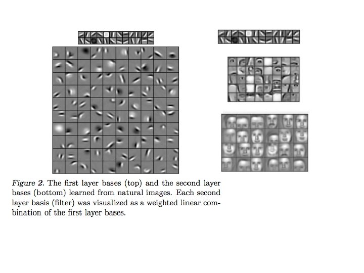
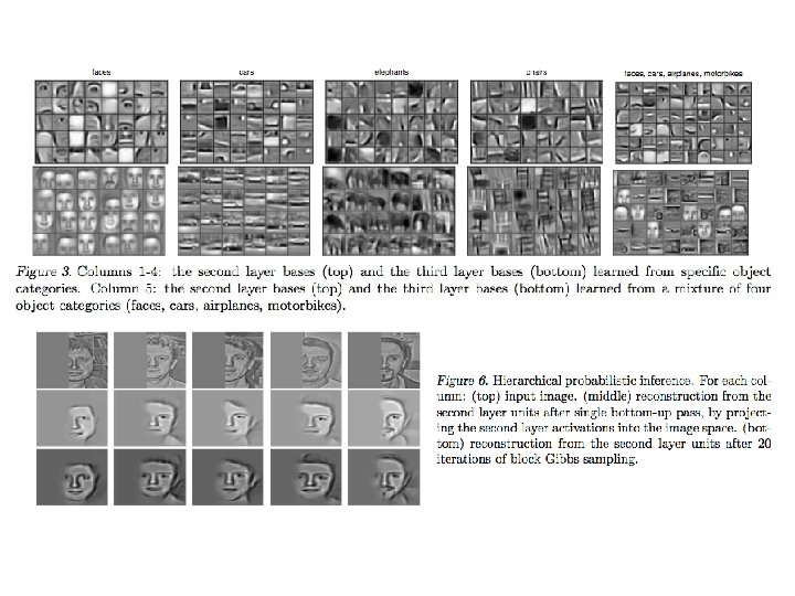
Convolutional Deep Belief net Honglak Lee, Roger Grosse, Rajesh Ranganath and Andrew Y. Ng. In Proceedings of the Twenty-Sixth International Conference on Machine Learning, 2009.

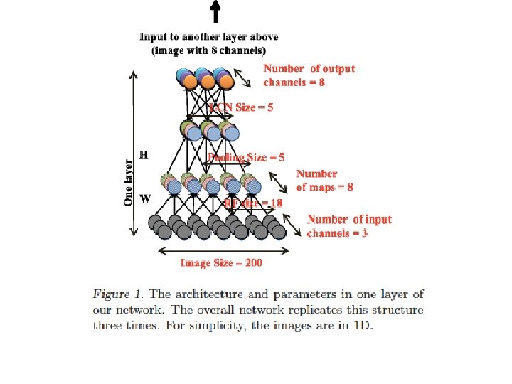
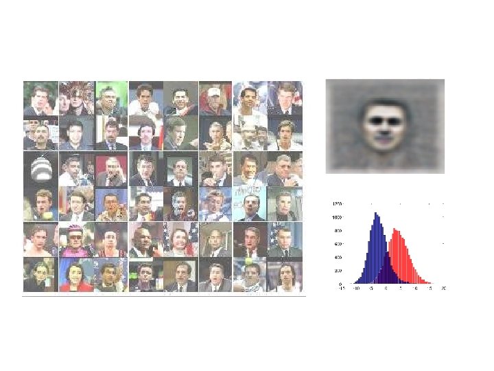
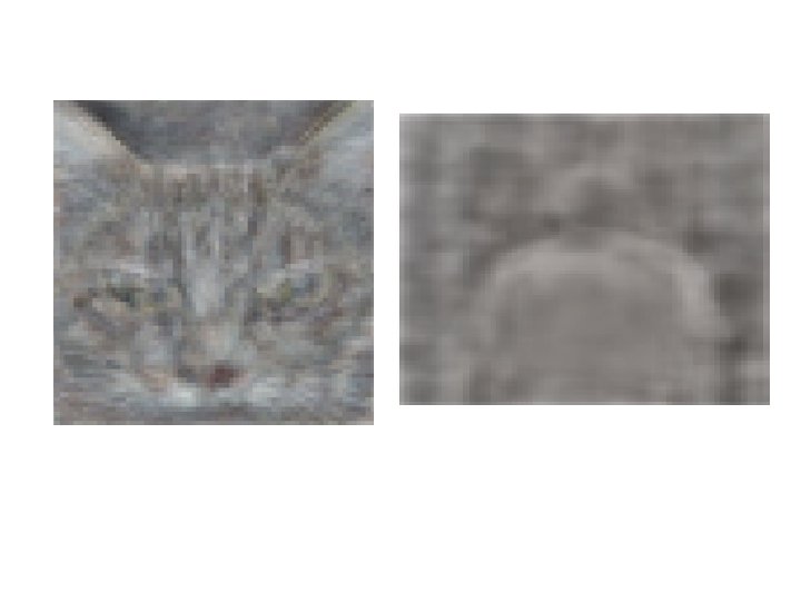
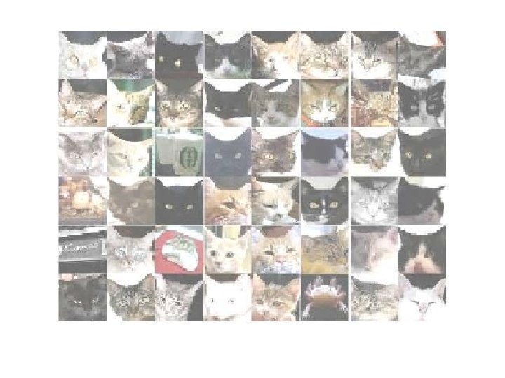
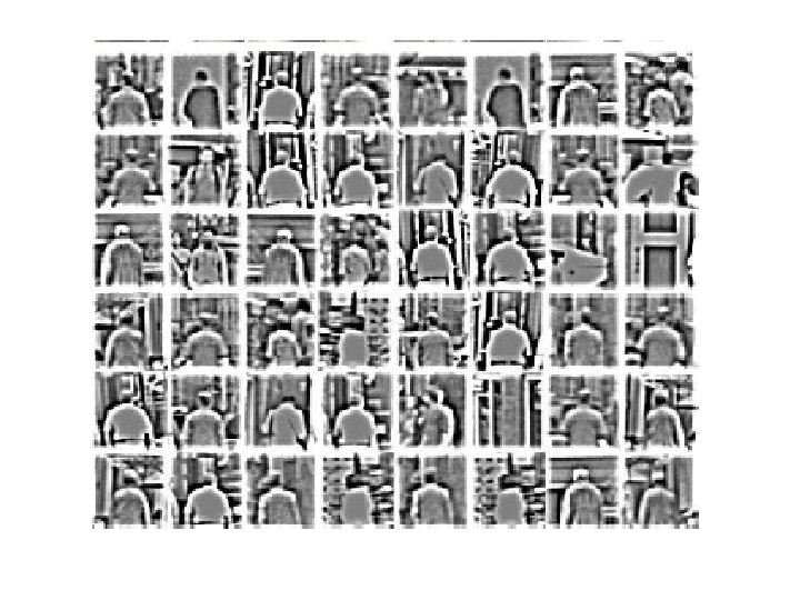
Large scale DBN • Building High-level Features Using Large Scale Unsupervised Learning Quoc V. Le, Marc’Aurelio Ranzato, Rajat Monga, Matthieu Devin, Kai Chen, Greg S. Corrado, J. Dean and Andrew Ng. • a 9 -layered locally connected sparse autoencoder with pooling and local contrast normalization on a large dataset of images • 1 billion connections, the dataset has 10 million 200 x 200 pixel images downloaded from the Internet. • Train on 1000 machines (16, 000 cores) for three days.
 Reducing the dimensionality of data with neural")
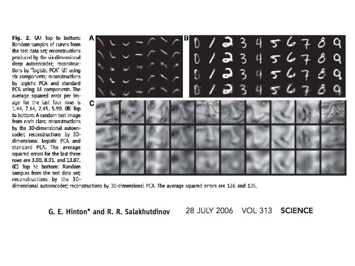
DBN deep autoencoder Hinton and Salakhutdinov (2006) Reducing the dimensionality of data with neural networks (Science 313, 504 -507)

A comparison of methods for compressing digit images to 30 real numbers. real data 30 -D deep auto 30 -D logistic PCA 30 -D PCA

The training and test sets for predicting face orientation 100, 500, or 1000 labeled cases 11, 000 unlabeled cases face patches from new people

Retrieving documents that are similar to a query document • We can use an auto-encoder to find low-dimensional codes for documents that allow fast and accurate retrieval of similar documents from a large set. • We start by converting each document into a “bag of words”. This a 2000 dimensional vector that contains the counts for each of the 2000 commonest words.

2000 reconstructed counts output vector 500 neurons 250 neurons 10 250 neurons 500 neurons 2000 word counts How to compress the count vector • We train the neural network to reproduce its input vector as its output • This forces it to compress as much information as possible into the 10 numbers in the central bottleneck. • These 10 numbers are then a good way to compare input documents. vector

Top layer only have two hidden nodes

First compress all documents to 2 numbers using a type of PCA Then use different colors for different document categories

First compress all documents to 2 numbers. Then use different colors for different document categories
- Slides: 48