Data Encoding Chapter 5 part 1 CSE 3213

Data Encoding – Chapter 5 (part 1) CSE 3213 Fall 2011 11/29/2020 5: 43 PM 1

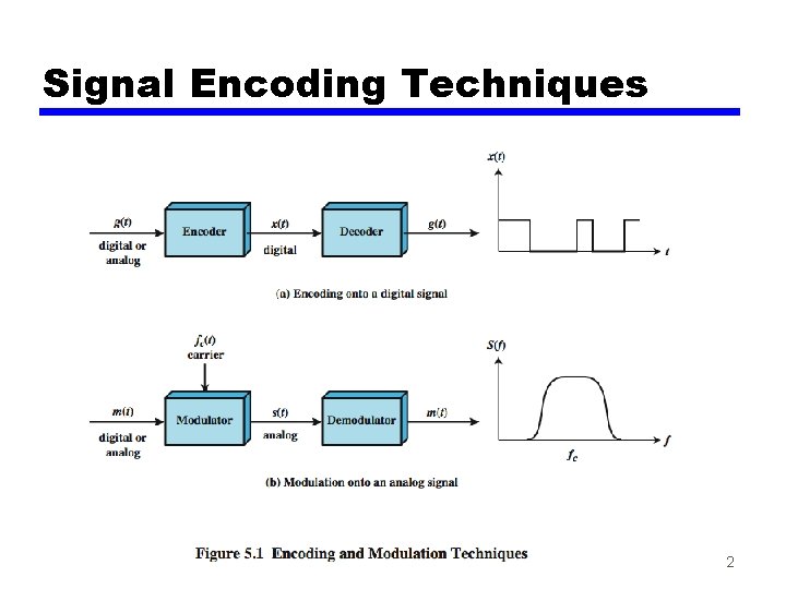
Signal Encoding Techniques 2

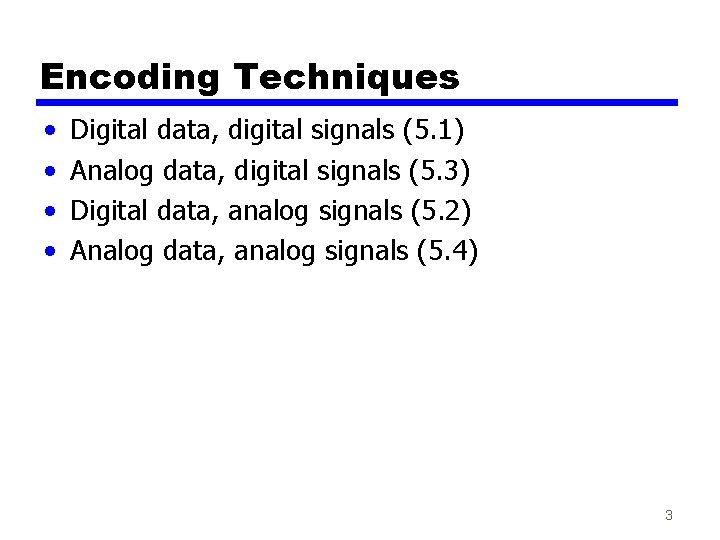
Encoding Techniques • • Digital data, digital signals (5. 1) Analog data, digital signals (5. 3) Digital data, analog signals (5. 2) Analog data, analog signals (5. 4) 3

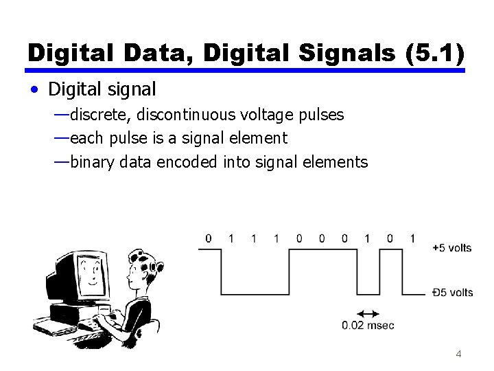
Digital Data, Digital Signals (5. 1) • Digital signal —discrete, discontinuous voltage pulses —each pulse is a signal element —binary data encoded into signal elements 4

Terminology (1) • Unipolar — all signal elements have same sign • Polar — one logic state represented by positive voltage the other by negative voltage • Data rate — rate of data transmission R, in bits per second • Duration or length of a bit — time taken for transmitter to emit the bit (1/R) 5

Terminology (2) • Modulation rate — rate at which the signal level changes — measured in baud = number of signal elements per second • Mark and Space — binary 1 and binary 0 respectively 6

Interpreting Signals • Need to know — timing of bits - when they start and end — signal levels • Factors affecting successful interpreting of signals — — signal to noise ratio data rate bandwidth encoding scheme 7

Comparison of Encoding Schemes (1) Factors to compare: • Signal Spectrum — lack of high frequencies reduces required bandwidth — concentrate power in the middle of the bandwidth • Clocking — synchronizing transmitter and receiver, using either • external clock, or • sync mechanism based on signal 8

Comparison of Encoding Schemes (2) • Error detection — responsibility of data link control — but can be built in to signal encoding for faster detection • Signal interference and noise immunity — some codes are better than others • Cost and complexity — higher signal rate ( and thus data rate) lead to higher costs — some codes require signal rate greater than data rate 9

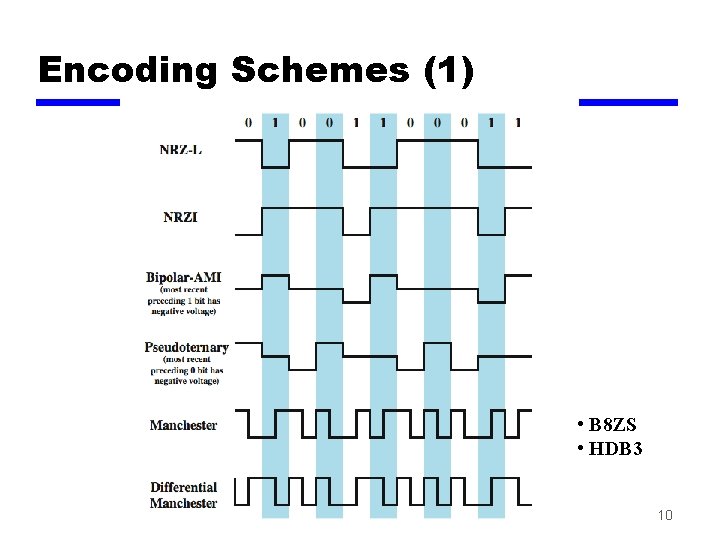
Encoding Schemes (1) • B 8 ZS • HDB 3 10

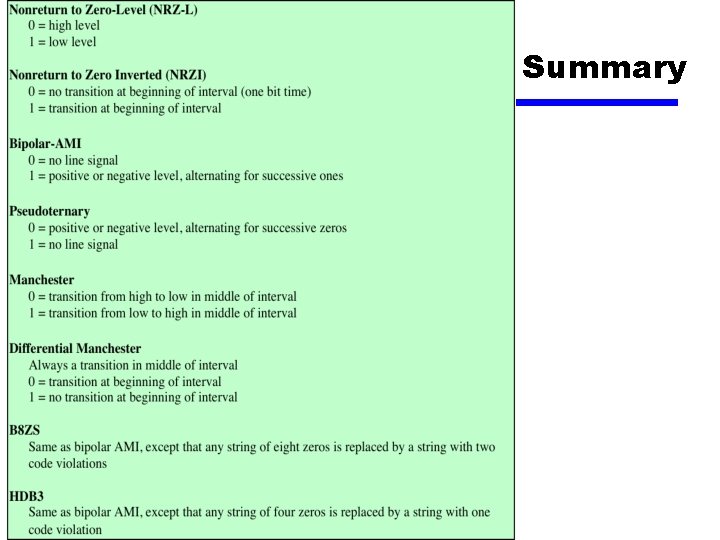
Encoding Schemes (2) • • Nonreturn to Zero-Level (NRZ-L) Nonreturn to Zero Inverted (NRZI) Bipolar -AMI Pseudoternary Manchester Differential Manchester B 8 ZS HDB 3 11

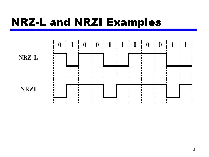
Nonreturn to Zero-Level (NRZ-L) • Two different voltages for 0 and 1 bits • Voltage constant during bit interval — no transition during a bit (no return to zero voltage) — absence of voltage for 0, constant positive voltage for 1 — more often, negative voltage for 1, and positive voltage for 0 (NRZ-L) 12

Nonreturn to Zero Inverted • Non-return to zero, inverted on ones • Constant voltage pulse for duration of bit • Data encoded as presence or absence of signal transition at beginning of bit time — transition (low to high or high to low) denotes a binary 1 — no transition denotes binary 0 • An example of differential encoding 13

NRZ-L and NRZI Examples 14

Differential Encoding • NRZI is an example of differential encoding • Data represented by changes rather than levels • More reliable detection of transition rather than levels • If the leads from an attached device to a twisted -pair lines are accidentally inverted, all 1 s and 0 s for NRZ-L will be inverted. This does not happen with differential encoding (NRZI). 15

NRZ pros and cons • Pros — easy to engineer — make good use of bandwidth • Cons — presence of a DC component — lack of synchronization capability • Used for magnetic recording • Not often used for signal transmission 16

Multilevel Binary • Use more than two signal levels — Bipolar-AMI (Alternate Mark Inversion) — Pseudoternary 17

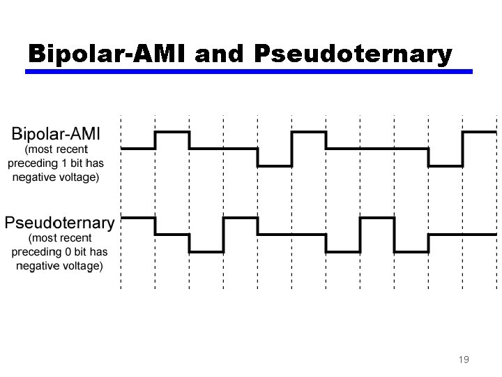
Bipolar-AMI • binary 0 represented by no line signal • binary 1 represented by positive or negative pulse • binary 1 pulses alternate in polarity • no loss of sync if a long string of 1 s occurs (long strings of 0 s still a problem) • no net DC component • lower bandwidth (than biphase coding) • easy error detection (due to pulse alternation) 18

Bipolar-AMI and Pseudoternary 19

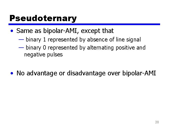
Pseudoternary • Same as bipolar-AMI, except that — binary 1 represented by absence of line signal — binary 0 represented by alternating positive and negative pulses • No advantage or disadvantage over bipolar-AMI 20

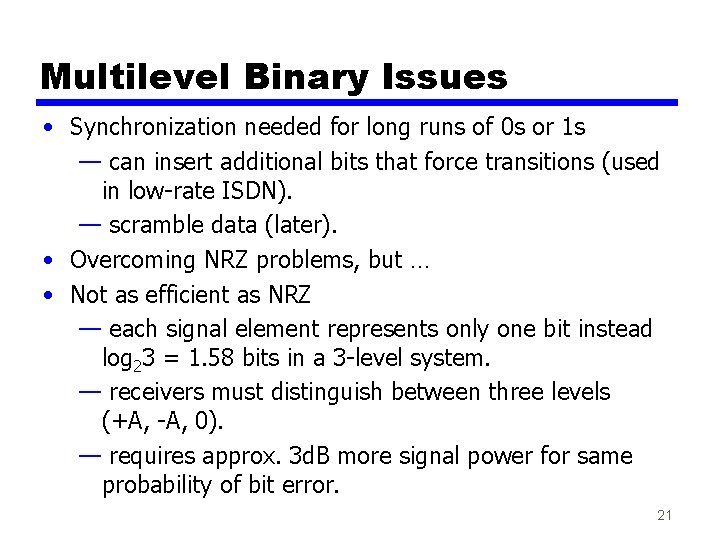
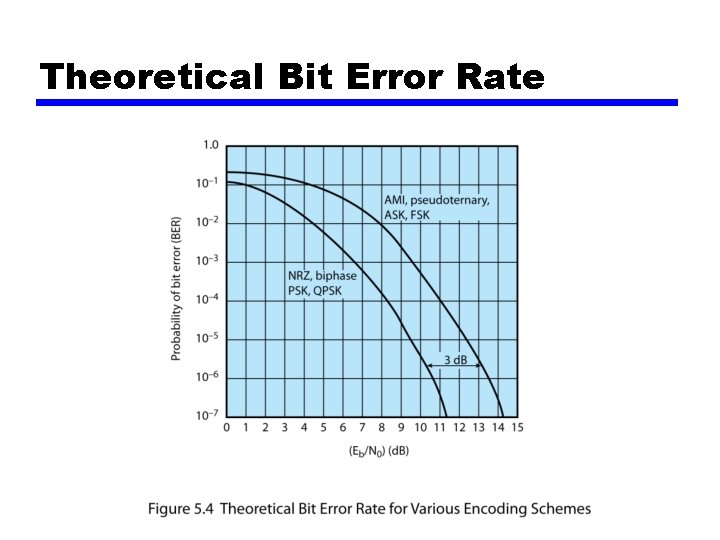
Multilevel Binary Issues • Synchronization needed for long runs of 0 s or 1 s — can insert additional bits that force transitions (used in low-rate ISDN). — scramble data (later). • Overcoming NRZ problems, but … • Not as efficient as NRZ — each signal element represents only one bit instead log 23 = 1. 58 bits in a 3 -level system. — receivers must distinguish between three levels (+A, -A, 0). — requires approx. 3 d. B more signal power for same probability of bit error. 21

Theoretical Bit Error Rate

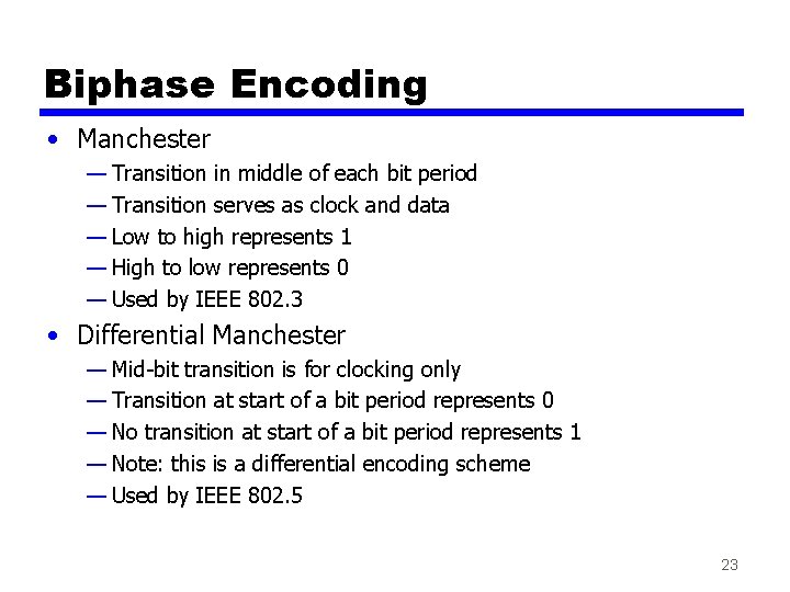
Biphase Encoding • Manchester — Transition in middle of each bit period — Transition serves as clock and data — Low to high represents 1 — High to low represents 0 — Used by IEEE 802. 3 • Differential Manchester — Mid-bit transition is for clocking only — Transition at start of a bit period represents 0 — No transition at start of a bit period represents 1 — Note: this is a differential encoding scheme — Used by IEEE 802. 5 23

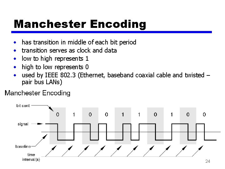
Manchester Encoding • • • has transition in middle of each bit period transition serves as clock and data low to high represents 1 high to low represents 0 used by IEEE 802. 3 (Ethernet, baseband coaxial cable and twisted – pair bus LANs) 24

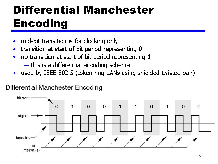
Differential Manchester Encoding • mid-bit transition is for clocking only • transition at start of bit period representing 0 • no transition at start of bit period representing 1 — this is a differential encoding scheme • used by IEEE 802. 5 (token ring LANs using shielded twisted pair) 25

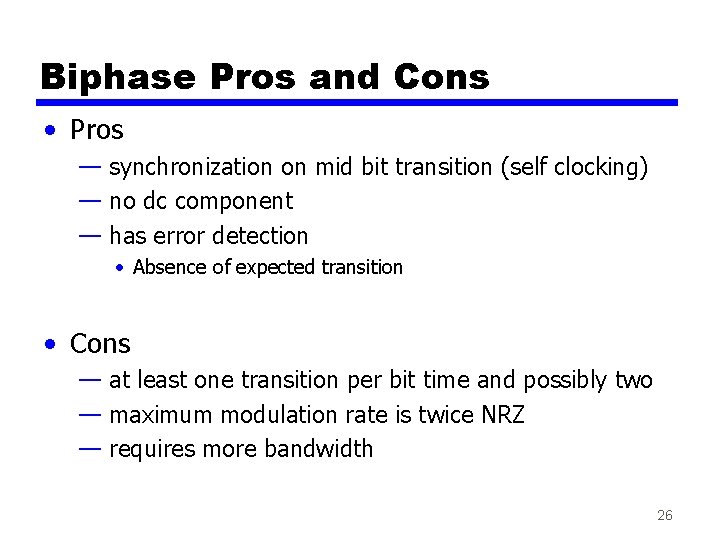
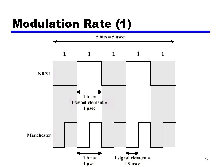
Biphase Pros and Cons • Pros — synchronization on mid bit transition (self clocking) — no dc component — has error detection • Absence of expected transition • Cons — at least one transition per bit time and possibly two — maximum modulation rate is twice NRZ — requires more bandwidth 26

Modulation Rate (1) 27

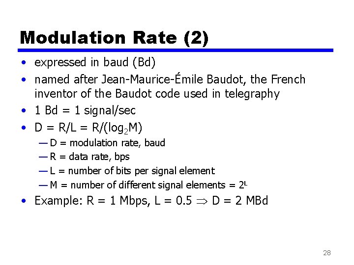
Modulation Rate (2) • expressed in baud (Bd) • named after Jean-Maurice-Émile Baudot, the French inventor of the Baudot code used in telegraphy • 1 Bd = 1 signal/sec • D = R/L = R/(log 2 M) — D = modulation rate, baud — R = data rate, bps — L = number of bits per signal element — M = number of different signal elements = 2 L • Example: R = 1 Mbps, L = 0. 5 D = 2 MBd 28

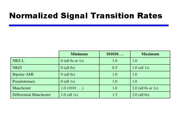
Normalized Signal Transition Rates Table 5. 3

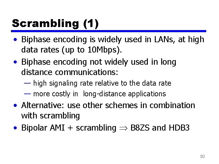
Scrambling (1) • Biphase encoding is widely used in LANs, at high data rates (up to 10 Mbps). • Biphase encoding not widely used in long distance communications: — high signaling rate relative to the data rate — more costly in long-distance applications • Alternative: use other schemes in combination with scrambling • Bipolar AMI + scrambling B 8 ZS and HDB 3 30

Scrambling (2) • Use scrambling to replace sequences that would produce constant voltage • These filling sequences must — produce enough transitions to sync — be recognized by receiver and replaced with original — be same length as original • Design goals — — have no DC component have no long sequences of zero level line signal have no reduction in data rate give error detection capability 31

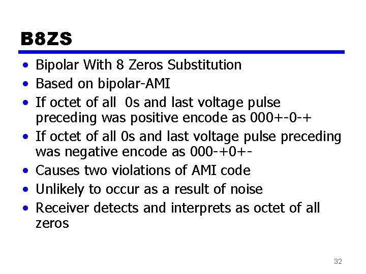
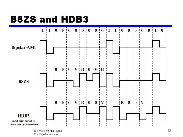
B 8 ZS • Bipolar With 8 Zeros Substitution • Based on bipolar-AMI • If octet of all 0 s and last voltage pulse preceding was positive encode as 000+-0 -+ • If octet of all 0 s and last voltage pulse preceding was negative encode as 000 -+0+ • Causes two violations of AMI code • Unlikely to occur as a result of noise • Receiver detects and interprets as octet of all zeros 32

B 8 ZS and HDB 3 33

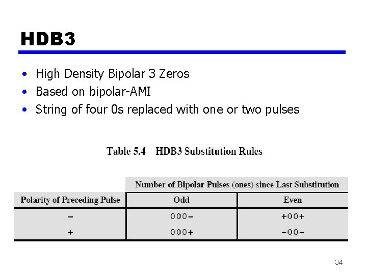
HDB 3 • High Density Bipolar 3 Zeros • Based on bipolar-AMI • String of four 0 s replaced with one or two pulses 34

Summary

Reading • Section 5. 1, Stallings’ book • Homework: problems 5. 6 to 5. 9, Stallings’ book 36