CSC 401 Analysis of Algorithms Lecture Notes 13

CSC 401 – Analysis of Algorithms Lecture Notes 13 Graphs: Concepts, Representation, and Traversal Objectives: • • • Introduce graphs Present data structures for graphs Discuss the graph connectivity Present the depth-first search algorithm Present the breath-first search algorithm 1

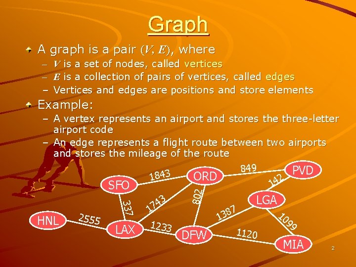
Graph A graph is a pair (V, E), where – – – V is a set of nodes, called vertices E is a collection of pairs of vertices, called edges Vertices and edges are positions and store elements Example: 337 HNL 2555 LAX 3 4 7 1 1233 802 – A vertex represents an airport and stores the three-letter airport code – An edge represents a flight route between two airports and stores the mileage of the route 849 PVD 3 ORD 184 2 14 SFO 7 138 DFW LGA 1120 10 99 MIA 2

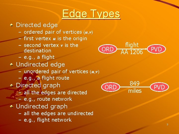
Edge Types Directed edge – – – ordered pair of vertices (u, v) first vertex u is the origin second vertex v is the destination – e. g. , a flight ORD flight AA 1206 PVD Undirected edge – unordered pair of vertices (u, v) – e. g. , a flight route Directed graph – all the edges are directed – e. g. , route network ORD 849 miles PVD Undirected graph – all the edges are undirected – e. g. , flight network 3

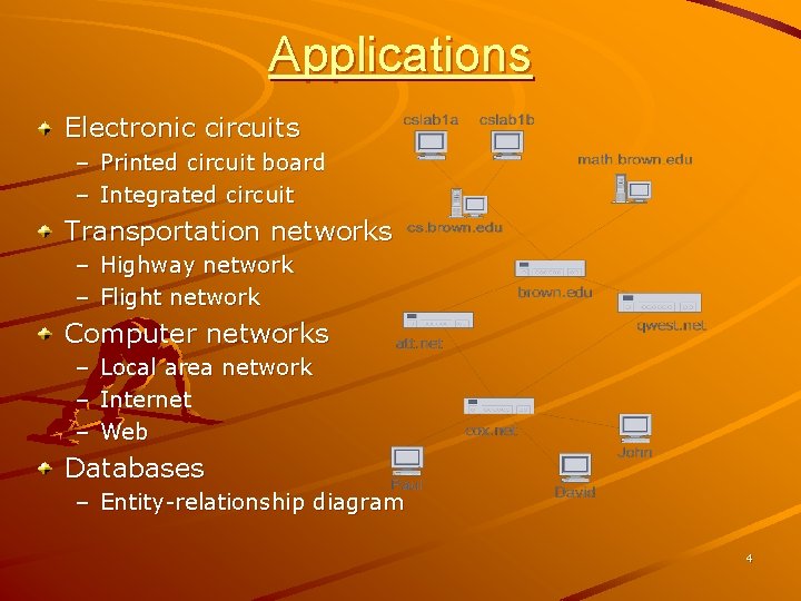
Applications Electronic circuits – Printed circuit board – Integrated circuit Transportation networks – Highway network – Flight network Computer networks – Local area network – Internet – Web Databases – Entity-relationship diagram 4

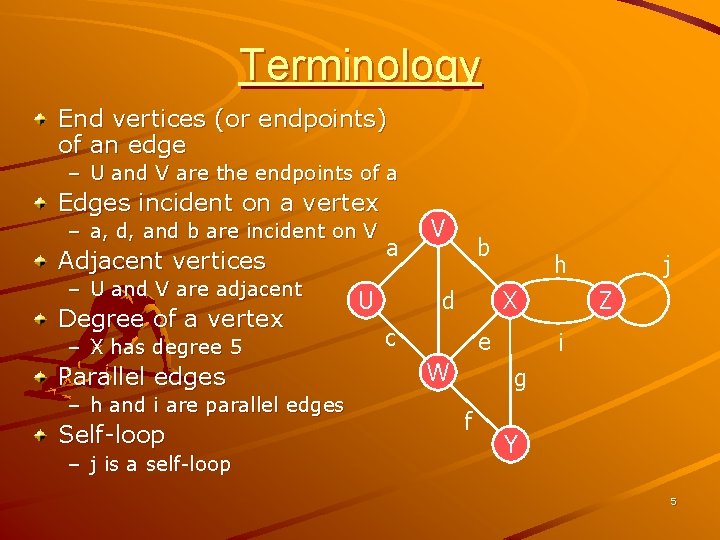
Terminology End vertices (or endpoints) of an edge – U and V are the endpoints of a Edges incident on a vertex – a, d, and b are incident on V Adjacent vertices – U and V are adjacent Degree of a vertex – X has degree 5 Parallel edges – h and i are parallel edges Self-loop – j is a self-loop a U V b d h X c e W j Z i g f Y 5

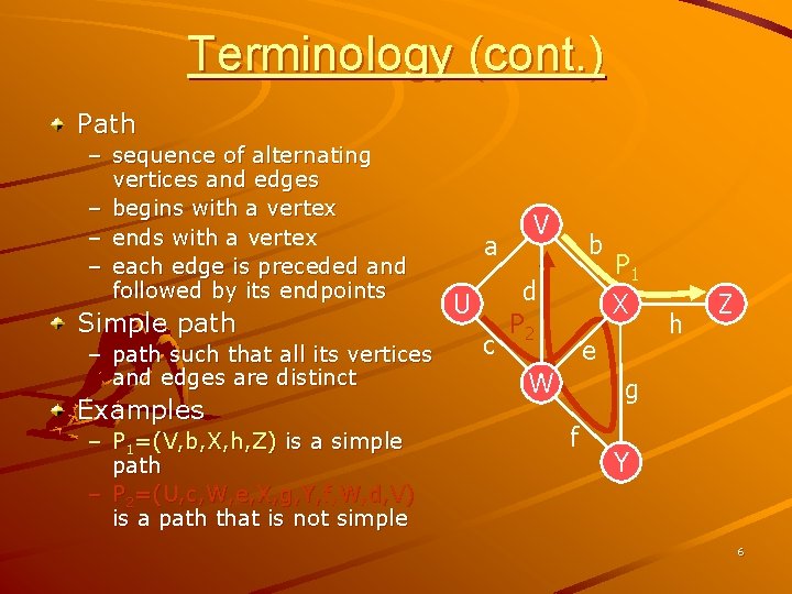
Terminology (cont. ) Path – sequence of alternating vertices and edges – begins with a vertex – ends with a vertex – each edge is preceded and followed by its endpoints Simple path – path such that all its vertices and edges are distinct Examples – P 1=(V, b, X, h, Z) is a simple path – P 2=(U, c, W, e, X, g, Y, f, W, d, V) is a path that is not simple a U c V b d P 2 P 1 X e W h Z g f Y 6

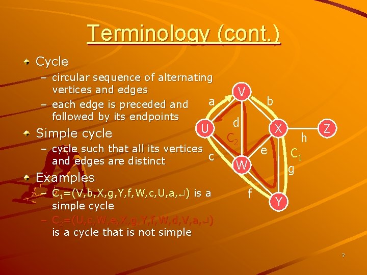
Terminology (cont. ) Cycle – circular sequence of alternating vertices and edges a – each edge is preceded and followed by its endpoints Simple cycle U – cycle such that all its vertices c and edges are distinct Examples – C 1=(V, b, X, g, Y, f, W, c, U, a, ) is a simple cycle – C 2=(U, c, W, e, X, g, Y, f, W, d, V, a, ) is a cycle that is not simple V b d C 2 X e C 1 g W f h Z Y 7

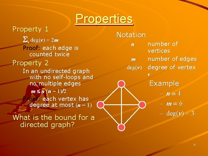
Property 1 Properties Sv deg(v) = 2 m Proof: each edge is counted twice Property 2 In an undirected graph with no self-loops and no multiple edges m n (n - 1)/2 Proof: each vertex has degree at most (n - 1) What is the bound for a directed graph? Notation n m deg(v) number of vertices number of edges degree of vertex v Example – n=4 – m=6 – deg(v) = 3 8

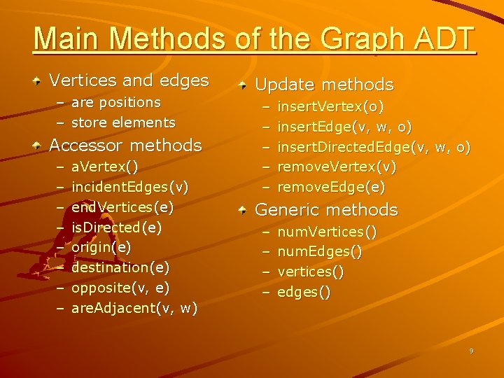
Main Methods of the Graph ADT Vertices and edges – are positions – store elements Accessor methods – – – – a. Vertex() incident. Edges(v) end. Vertices(e) is. Directed(e) origin(e) destination(e) opposite(v, e) are. Adjacent(v, w) Update methods – – – insert. Vertex(o) insert. Edge(v, w, o) insert. Directed. Edge(v, w, o) remove. Vertex(v) remove. Edge(e) Generic methods – – num. Vertices() num. Edges() vertices() edges() 9

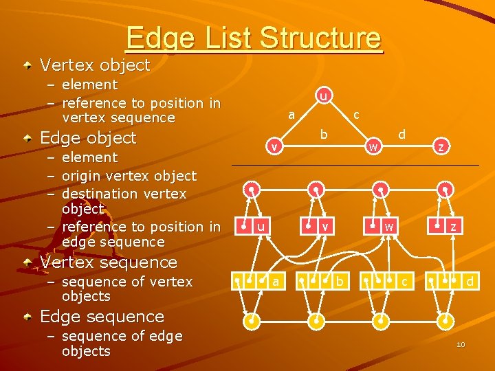
Edge List Structure Vertex object – element – reference to position in vertex sequence u a Edge object – element – origin vertex object – destination vertex object – reference to position in edge sequence v u c b d w z w v z Vertex sequence – sequence of vertex objects a b c d Edge sequence – sequence of edge objects 10

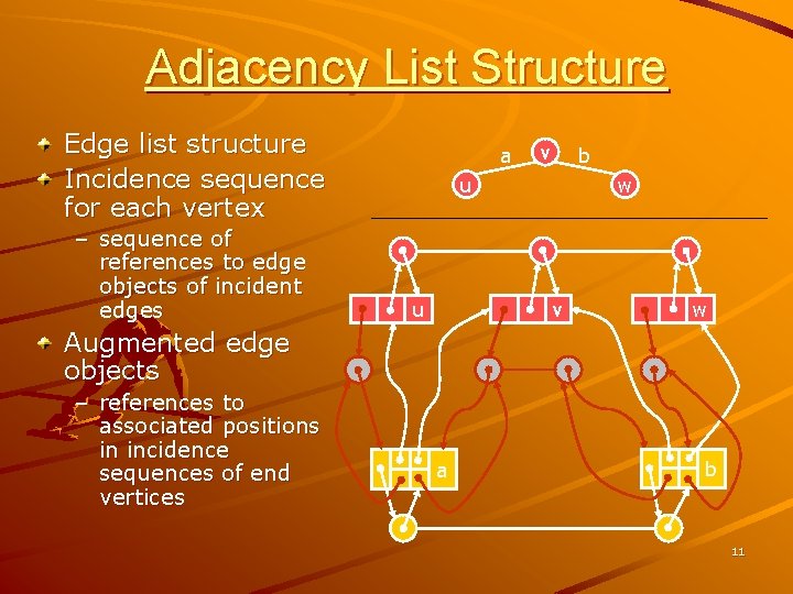
Adjacency List Structure Edge list structure Incidence sequence for each vertex – sequence of references to edge objects of incident edges a v b u u w v w Augmented edge objects – references to associated positions in incidence sequences of end vertices a b 11

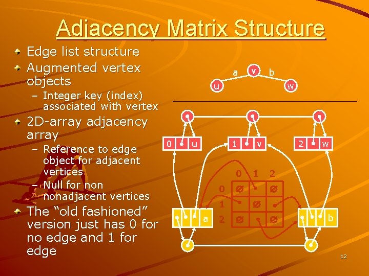
Adjacency Matrix Structure Edge list structure Augmented vertex objects a – Reference to edge object for adjacent vertices – Null for nonadjacent vertices The “old fashioned” version just has 0 for no edge and 1 for edge b u – Integer key (index) associated with vertex 2 D-array adjacency array v 0 u w 1 0 0 2 1 w 2 1 a 2 v b 12

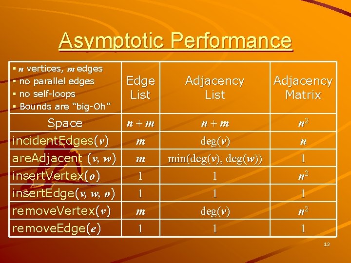
Asymptotic Performance § n vertices, m edges § no parallel edges § no self-loops § Bounds are “big-Oh” Edge List n+m Space incident. Edges(v) m are. Adjacent (v, w) m insert. Vertex(o) 1 insert. Edge(v, w, o) 1 remove. Vertex(v) remove. Edge(e) m 1 Adjacency List Adjacency Matrix n+m deg(v) min(deg(v), deg(w)) 1 n 2 n 1 n 2 1 deg(v) 1 1 n 2 1 13

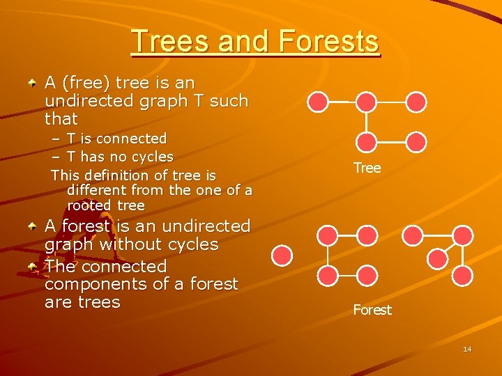
Trees and Forests A (free) tree is an undirected graph T such that – T is connected – T has no cycles This definition of tree is different from the one of a rooted tree A forest is an undirected graph without cycles The connected components of a forest are trees Tree Forest 14

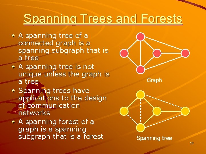
Spanning Trees and Forests A spanning tree of a connected graph is a spanning subgraph that is a tree A spanning tree is not unique unless the graph is a tree Spanning trees have applications to the design of communication networks A spanning forest of a graph is a spanning subgraph that is a forest Graph Spanning tree 15

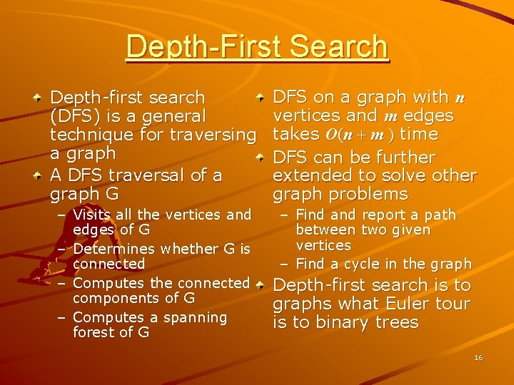
Depth-First Search Depth-first search (DFS) is a general technique for traversing a graph A DFS traversal of a graph G DFS on a graph with n vertices and m edges takes O(n + m ) time DFS can be further extended to solve other graph problems – Visits all the vertices and edges of G – Determines whether G is connected – Computes the connected components of G – Computes a spanning forest of G – Find and report a path between two given vertices – Find a cycle in the graph Depth-first search is to graphs what Euler tour is to binary trees 16

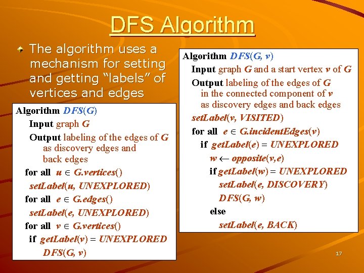
DFS Algorithm The algorithm uses a mechanism for setting and getting “labels” of vertices and edges Algorithm DFS(G) Input graph G Output labeling of the edges of G as discovery edges and back edges for all u G. vertices() set. Label(u, UNEXPLORED) for all e G. edges() set. Label(e, UNEXPLORED) for all v G. vertices() if get. Label(v) = UNEXPLORED DFS(G, v) Algorithm DFS(G, v) Input graph G and a start vertex v of G Output labeling of the edges of G in the connected component of v as discovery edges and back edges set. Label(v, VISITED) for all e G. incident. Edges(v) if get. Label(e) = UNEXPLORED w opposite(v, e) if get. Label(w) = UNEXPLORED set. Label(e, DISCOVERY) DFS(G, w) else set. Label(e, BACK) 17

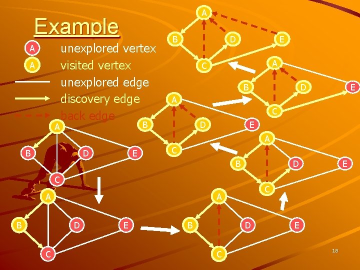
A Example A A A unexplored vertex visited vertex unexplored edge discovery edge back edge B D E A C B D E A B D E C B D C A B C C A D E B D C E E 18

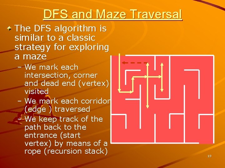
DFS and Maze Traversal The DFS algorithm is similar to a classic strategy for exploring a maze – We mark each intersection, corner and dead end (vertex) visited – We mark each corridor (edge ) traversed – We keep track of the path back to the entrance (start vertex) by means of a rope (recursion stack) 19

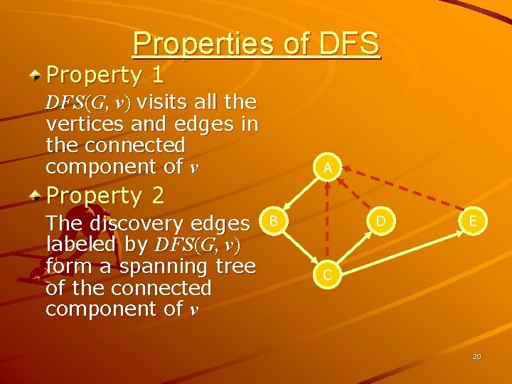
Properties of DFS Property 1 DFS(G, v) visits all the vertices and edges in the connected component of v A Property 2 The discovery edges labeled by DFS(G, v) form a spanning tree of the connected component of v B D E C 20

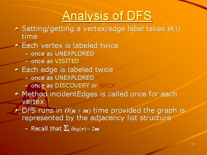
Analysis of DFS Setting/getting a vertex/edge label takes O(1) time Each vertex is labeled twice – once as UNEXPLORED – once as VISITED Each edge is labeled twice – once as UNEXPLORED – once as DISCOVERY or BACK Method incident. Edges is called once for each vertex DFS runs in O(n + m) time provided the graph is represented by the adjacency list structure – Recall that Sv deg(v) = 2 m 21

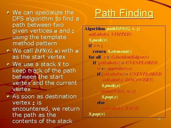
Path Finding We can specialize the DFS algorithm to find a path between two Algorithm path. DFS(G, v, z) given vertices u and z set. Label(v, VISITED) using the template S. push(v) method pattern if v = z We call DFS(G, u) with u return S. elements() for all e G. incident. Edges(v) as the start vertex if get. Label(e) = UNEXPLORED We use a stack S to w opposite(v, e) keep track of the path if get. Label(w) = UNEXPLORED between the start set. Label(e, DISCOVERY) vertex and the current S. push(e) vertex path. DFS(G, w, z) S. pop(e) As soon as destination else vertex z is set. Label(e, BACK) encountered, we return S. pop(v) the path as the 22 contents of the stack

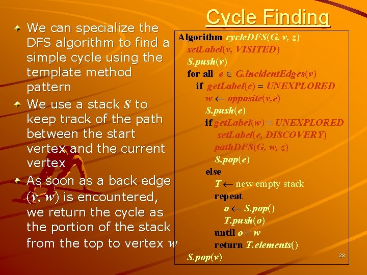
Cycle Finding We can specialize the Algorithm cycle. DFS(G, v, z) DFS algorithm to find a set. Label(v, VISITED) simple cycle using the S. push(v) template method for all e G. incident. Edges(v) if get. Label(e) = UNEXPLORED pattern w opposite(v, e) We use a stack S to S. push(e) keep track of the path if get. Label(w) = UNEXPLORED between the start set. Label(e, DISCOVERY) path. DFS(G, w, z) vertex and the current S. pop(e) vertex else As soon as a back edge T new empty stack repeat (v, w) is encountered, o S. pop() we return the cycle as T. push(o) the portion of the stack until o = w from the top to vertex w return T. elements() S. pop(v) 23

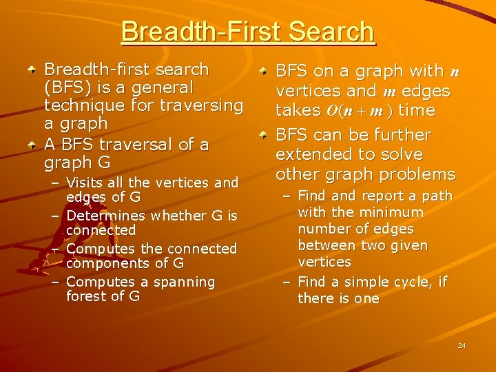
Breadth-First Search Breadth-first search (BFS) is a general technique for traversing a graph A BFS traversal of a graph G – Visits all the vertices and edges of G – Determines whether G is connected – Computes the connected components of G – Computes a spanning forest of G BFS on a graph with n vertices and m edges takes O(n + m ) time BFS can be further extended to solve other graph problems – Find and report a path with the minimum number of edges between two given vertices – Find a simple cycle, if there is one 24

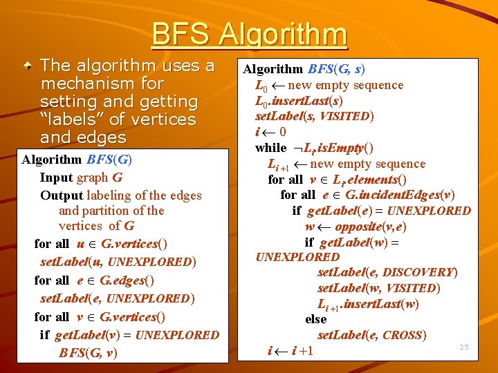
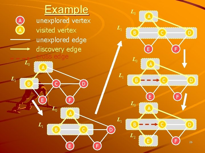
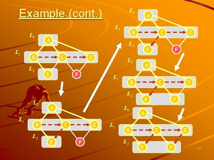
BFS Algorithm The algorithm uses a mechanism for setting and getting “labels” of vertices and edges Algorithm BFS(G) Input graph G Output labeling of the edges and partition of the vertices of G for all u G. vertices() set. Label(u, UNEXPLORED) for all e G. edges() set. Label(e, UNEXPLORED) for all v G. vertices() if get. Label(v) = UNEXPLORED BFS(G, v) Algorithm BFS(G, s) L 0 new empty sequence L 0. insert. Last(s) set. Label(s, VISITED) i 0 while Li. is. Empty() Li +1 new empty sequence for all v Li. elements() for all e G. incident. Edges(v) if get. Label(e) = UNEXPLORED w opposite(v, e) if get. Label(w) = UNEXPLORED set. Label(e, DISCOVERY) set. Label(w, VISITED) Li +1. insert. Last(w) else set. Label(e, CROSS) 25 i i +1

Example A A L 0 L 1 L 0 unexplored vertex visited vertex unexplored edge discovery edge cross edge L 1 B L 0 L 1 C E L 1 D A B L 1 C E A B L 0 D C F D F A B L 2 D F E F L 0 C E A B A C E D F 26

L 0 Example (cont. ) L 1 L 0 L 1 A B C L 2 A D E F E L 0 L 1 A B B L 2 L 0 C E D F L 1 F A C L 2 L 0 D E F A B L 2 D C E D F 27

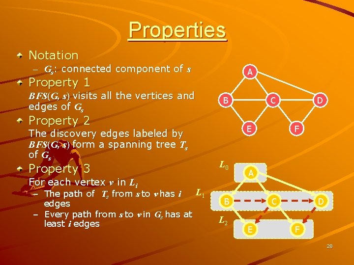
Properties Notation – Gs: connected component of s A Property 1 BFS(G, s) visits all the vertices and edges of Gs B Property 2 The discovery edges labeled by BFS(G, s) form a spanning tree Ts of Gs Property 3 E L 0 For each vertex v in Li L 1 – The path of Ts from s to v has i edges – Every path from s to v in Gs has at least i edges C F A B L 2 D C E D F 28

Analysis Setting/getting a vertex/edge label takes O(1) time Each vertex is labeled twice – once as UNEXPLORED – once as VISITED Each edge is labeled twice – once as UNEXPLORED – once as DISCOVERY or CROSS Each vertex is inserted once into a sequence Li Method incident. Edges is called once for each vertex BFS runs in O(n + m) time provided the graph is represented by the adjacency list structure – Recall that Sv deg(v) = 2 m 29

Applications Using the template method pattern, we can specialize the BFS traversal of a graph G to solve the following problems in O(n + m) time – Compute the connected components of G – Compute a spanning forest of G – Find a simple cycle in G, or report that G is a forest – Given two vertices of G, find a path in G between them with the minimum number of edges, or report that no such path exists 30

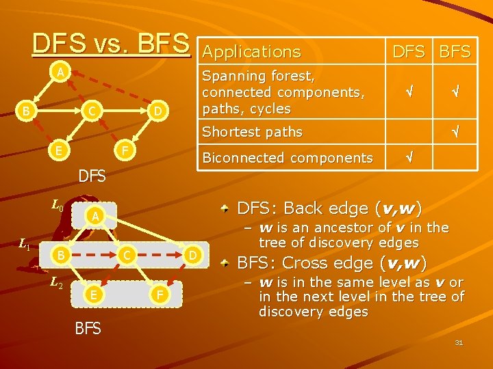
DFS vs. BFS A B C Applications Spanning forest, connected components, paths, cycles D DFS BFS Shortest paths E F Biconnected components DFS L 0 L 1 L 2 C E BFS DFS: Back edge (v, w) A B D F – w is an ancestor of v in the tree of discovery edges BFS: Cross edge (v, w) – w is in the same level as v or in the next level in the tree of discovery edges 31