csc 2535 2013 Lecture 8 Modeling image covariance

csc 2535 2013 Lecture 8 Modeling image covariance structure Geoffrey Hinton

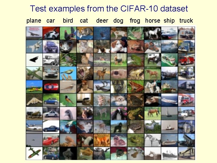
Test examples from the CIFAR-10 dataset plane car bird cat deer dog frog horse ship truck

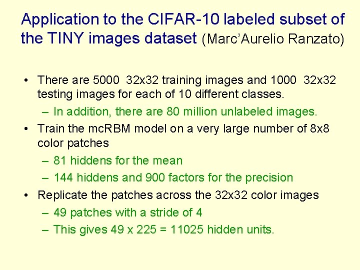
Application to the CIFAR-10 labeled subset of the TINY images dataset (Marc’Aurelio Ranzato) • There are 5000 32 x 32 training images and 1000 32 x 32 testing images for each of 10 different classes. – In addition, there are 80 million unlabeled images. • Train the mc. RBM model on a very large number of 8 x 8 color patches – 81 hiddens for the mean – 144 hiddens and 900 factors for the precision • Replicate the patches across the 32 x 32 color images – 49 patches with a stride of 4 – This gives 49 x 225 = 11025 hidden units.

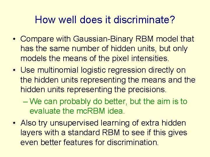
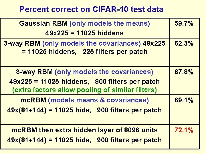
How well does it discriminate? • Compare with Gaussian-Binary RBM model that has the same number of hidden units, but only models the means of the pixel intensities. • Use multinomial logistic regression directly on the hidden units representing the means and the hidden units representing the precisions. – We can probably do better, but the aim is to evaluate the mc. RBM idea. • Also try unsupervised learning of extra hidden layers with a standard RBM to see if this gives even better features for discrimination.

Change of Topic • Modeling the covariance structure of image patches

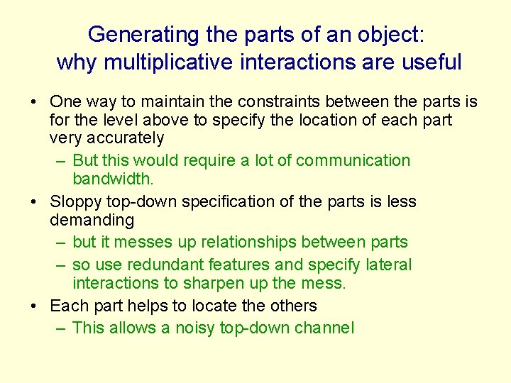
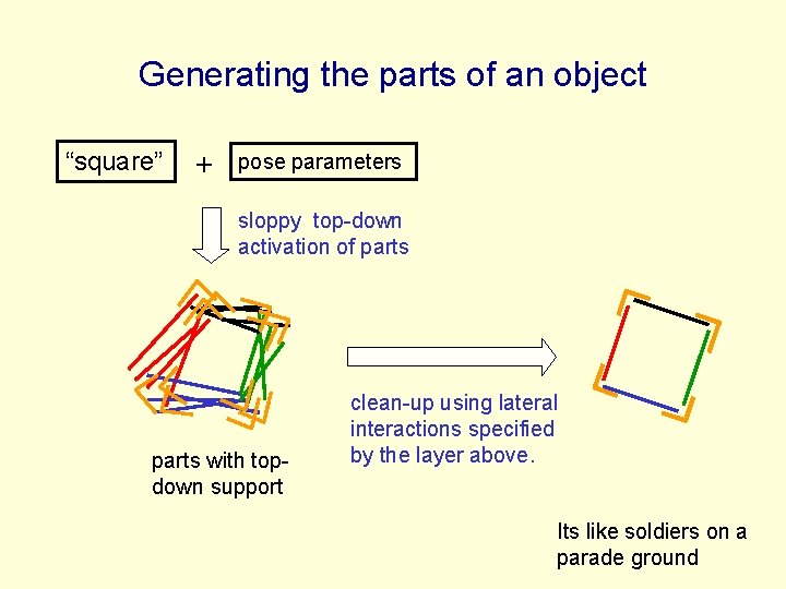
Generating the parts of an object: why multiplicative interactions are useful • One way to maintain the constraints between the parts is for the level above to specify the location of each part very accurately – But this would require a lot of communication bandwidth. • Sloppy top-down specification of the parts is less demanding – but it messes up relationships between parts – so use redundant features and specify lateral interactions to sharpen up the mess. • Each part helps to locate the others – This allows a noisy top-down channel

Generating the parts of an object “square” + pose parameters sloppy top-down activation of parts with topdown support clean-up using lateral interactions specified by the layer above. Its like soldiers on a parade ground

Towards a more powerful, multi-linear stackable learning module • We want the states of the units in one layer to modulate the pair-wise interactions in the layer below (not just the biases) – Can we do this without losing the nice property that the hidden units are conditionally independent given the visible states?

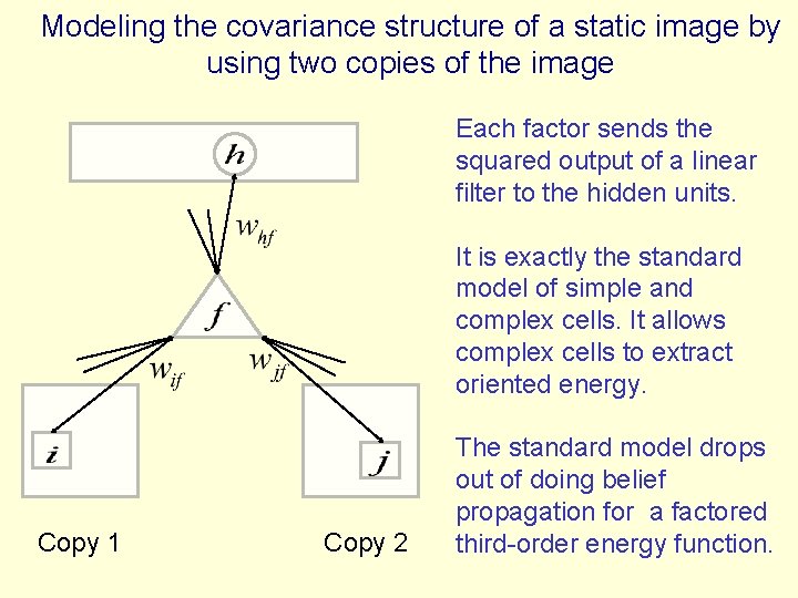
Modeling the covariance structure of a static image by using two copies of the image Each factor sends the squared output of a linear filter to the hidden units. It is exactly the standard model of simple and complex cells. It allows complex cells to extract oriented energy. Copy 1 Copy 2 The standard model drops out of doing belief propagation for a factored third-order energy function.

What is a vertical edge? • • • An intensity difference? A color difference? A texture difference? A depth difference? A motion difference? A combination of several of these? • Is there a single simple definition of a vertical edge that covers all of these cases?

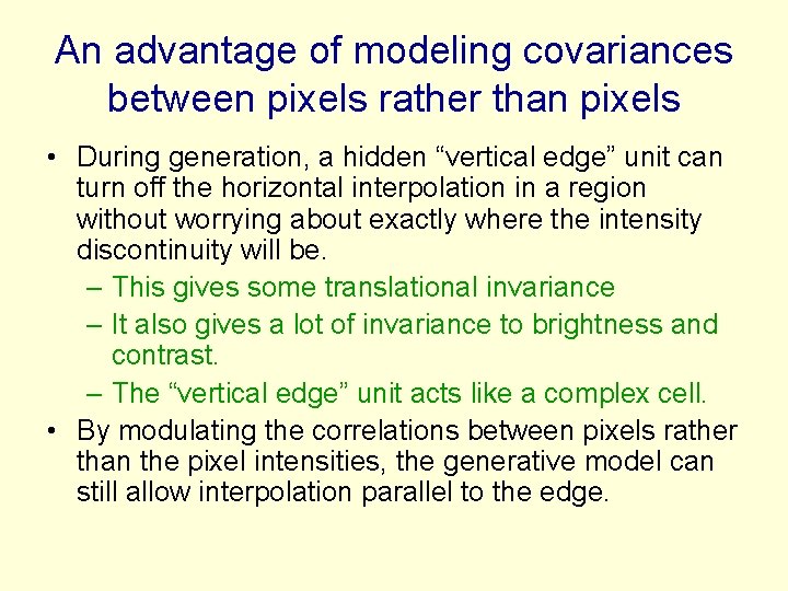
An advantage of modeling covariances between pixels rather than pixels • During generation, a hidden “vertical edge” unit can turn off the horizontal interpolation in a region without worrying about exactly where the intensity discontinuity will be. – This gives some translational invariance – It also gives a lot of invariance to brightness and contrast. – The “vertical edge” unit acts like a complex cell. • By modulating the correlations between pixels rather than the pixel intensities, the generative model can still allow interpolation parallel to the edge.

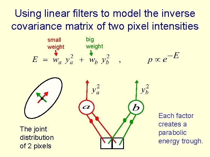
Using linear filters to model the inverse covariance matrix of two pixel intensities small weight The joint distribution of 2 pixels big weight Each factor creates a parabolic energy trough.

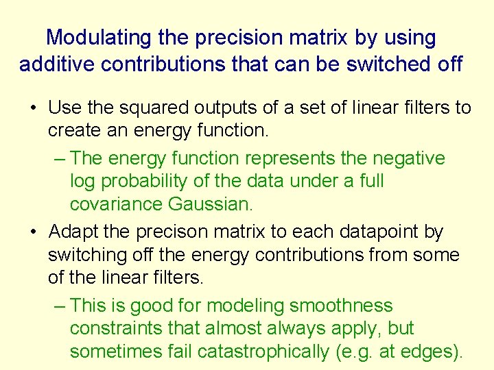
Modulating the precision matrix by using additive contributions that can be switched off • Use the squared outputs of a set of linear filters to create an energy function. – The energy function represents the negative log probability of the data under a full covariance Gaussian. • Adapt the precison matrix to each datapoint by switching off the energy contributions from some of the linear filters. – This is good for modeling smoothness constraints that almost always apply, but sometimes fail catastrophically (e. g. at edges).

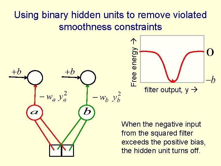
Free energy Using binary hidden units to remove violated smoothness constraints filter output, y When the negative input from the squared filter exceeds the positive bias, the hidden unit turns off.

Inference with hidden units that represent active smoothness constraints • The hidden units are all independent given the pixel intensities – The factors do not create dependencies between hidden units. • Given the states of the hidden units, the pixel intensity distribution is a full covariance Gaussian that is adapted for that particular image. – The hidden states do create dependencies between the pixels.

Learning with an adaptive precision matrix • Since the pixel intensities are no longer independent given the hidden states, it is much harder to produce reconstructions. – We could invert the precision matrix for each training example, but this is slow. • Instead, we produce reconstructions using Hybrid Monte Carlo, starting at the data. – The rest of the learning algorithm is the same as before.

Hybrid Monte Carlo • Given the pixel intensities, we can integrate out the hidden states to get a free energy that is a deterministic function of the image. – Backpropagation can then be used to get the derivatives of the free energy with respect to the pixel intensities. • Hybrid Monte Carlo simulates a particle that starts at the datapoint with a random initial momentum and then moves over the free energy surface. – 20 leapfrog steps work well for our networks.

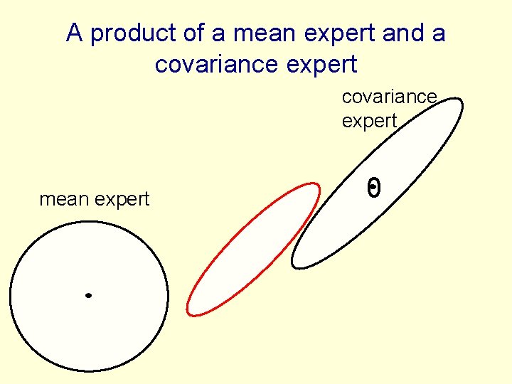
mc. RBM (mean and covariance RBM) • Use one set of binary hidden units to model the means of the real-valued pixels. – These hidden units learn blurry patterns for coloring in regions • Use a separate set of binary hidden units to model the image-specific precision matrix. – These hidden units get their input from factors. – The factors learn sharp edge filters for representing breakdowns in smoothness.

A product of a mean expert and a covariance expert mean expert 0

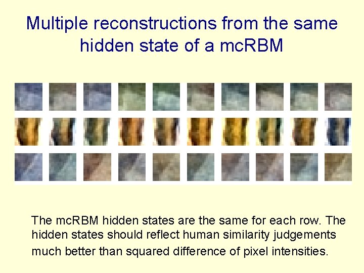
Multiple reconstructions from the same hidden state of a mc. RBM The mc. RBM hidden states are the same for each row. The hidden states should reflect human similarity judgements much better than squared difference of pixel intensities.

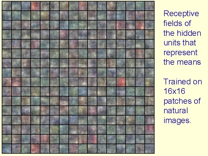
Receptive fields of the hidden units that represent the means Trained on 16 x 16 patches of natural images.

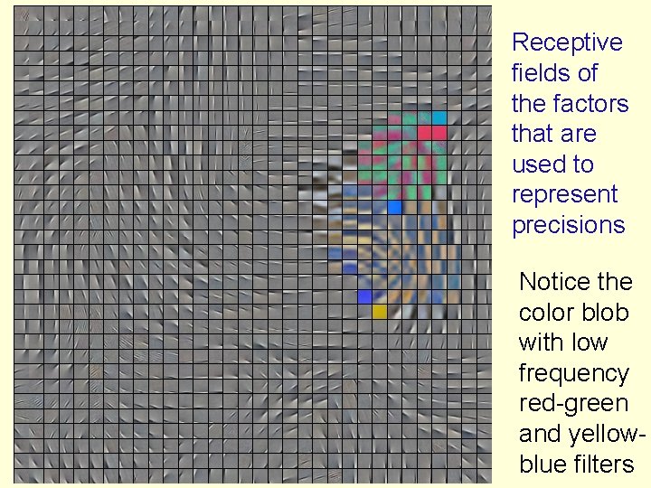
Receptive fields of the factors that are used to represent precisions Notice the color blob with low frequency red-green and yellowblue filters

Why is the map topographic? • We laid out the factors in a 2 -D grid and then connected each hidden unit to a small set of nearby factors. • If two factors get activated at the same time, it pays to connect them to the same hidden unit. – You only lose once by turning off that hidden unit.

Summary • RBM’s can be modified to allow factored multiplicative interactions. Inference is still easy. – Learning is still easy if we condition on one set of inputs (the pre-image for learning image transformations; the style for learning mocap) • Multiplicative interactions allow an RBM to model pixel covariances within one image in an image-specific way. – Unbiased reconstructions from the hidden units are hard to compute because we need to invert a precision matrix. – We can avoid the inversion by using Hybrid Monte Carlo in image space.

Percent correct on CIFAR-10 test data Gaussian RBM (only models the means) 49 x 225 = 11025 hiddens 3 -way RBM (only models the covariances) 49 x 225 = 11025 hiddens, 225 filters per patch 59. 7% 3 -way RBM (only models the covariances) 49 x 225 = 11025 hiddens, 900 filters per patch (extra factors allow pooling of similar filters) 67. 8% mc. RBM (models means & covariances) 49 x(81+144) = 11025 hids, 900 filters per patch 69. 1% mc. RBM then extra hidden layer of 8096 units 49 x(81+144) = 11025 hids, 900 filters per patch 72. 1% 62. 3%