CS 6220 DATA MINING TECHNIQUES Chapter 89 Classification

CS 6220: DATA MINING TECHNIQUES Chapter 8&9: Classification: Part 3 Instructor: Yizhou Sun yzsun@ccs. neu. edu October 30, 2020

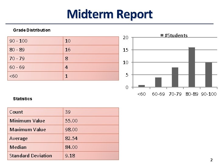
Midterm Report Grade Distribution 90 - 100 10 80 - 89 16 70 - 79 8 60 - 69 4 <60 1 15 10 5 0 Statistics Count 39 Minimum Value 55. 00 Maximum Value 98. 00 Average 82. 54 Median 84. 00 Standard Deviation 9. 18 #Students 20 <60 60 -69 70 -79 80 -89 90 -100 2

Announcement • Midterm Solution • https: //blackboard. neu. edu/bbcswebdav/pid-12532 -dt-wiki-rid -8320466_1/courses/CS 6220. 32435. 201330/mid_term. pdf • Course Project: • Midterm report due next week • A draft for final report • Don’t forget your project title • Main purpose • Check the progress and make sure you can finish it by the deadline 3

Chapter 8&9. Classification: Part 3 • Bayesian Learning • Naïve Bayes • Bayesian Belief Network • Instance-Based Learning • Summary 4

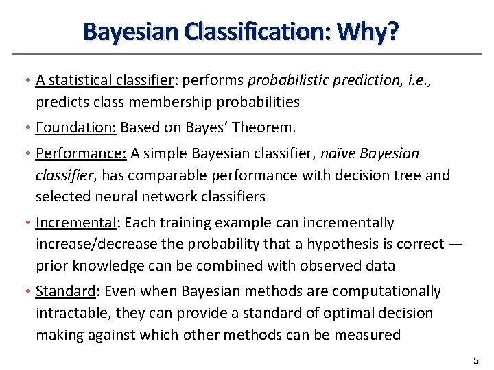
Bayesian Classification: Why? • A statistical classifier: performs probabilistic prediction, i. e. , predicts class membership probabilities • Foundation: Based on Bayes’ Theorem. • Performance: A simple Bayesian classifier, naïve Bayesian classifier, has comparable performance with decision tree and selected neural network classifiers • Incremental: Each training example can incrementally increase/decrease the probability that a hypothesis is correct — prior knowledge can be combined with observed data • Standard: Even when Bayesian methods are computationally intractable, they can provide a standard of optimal decision making against which other methods can be measured 5

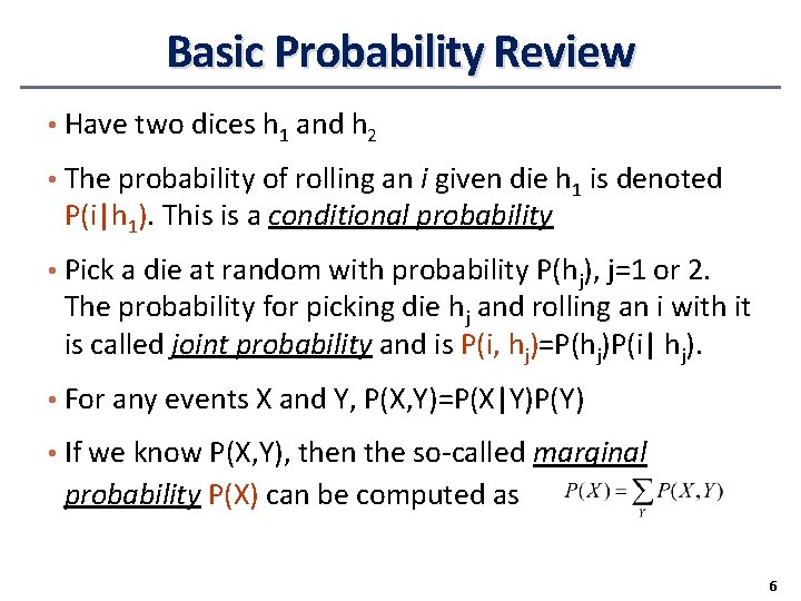
Basic Probability Review • Have two dices h 1 and h 2 • The probability of rolling an i given die h 1 is denoted P(i|h 1). This is a conditional probability • Pick a die at random with probability P(hj), j=1 or 2. The probability for picking die hj and rolling an i with it is called joint probability and is P(i, hj)=P(hj)P(i| hj). • For any events X and Y, P(X, Y)=P(X|Y)P(Y) • If we know P(X, Y), then the so-called marginal probability P(X) can be computed as 6

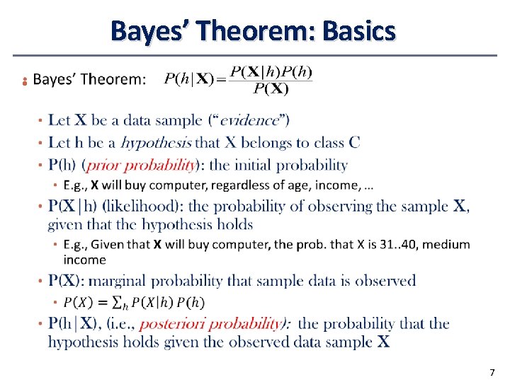
Bayes’ Theorem: Basics • 7

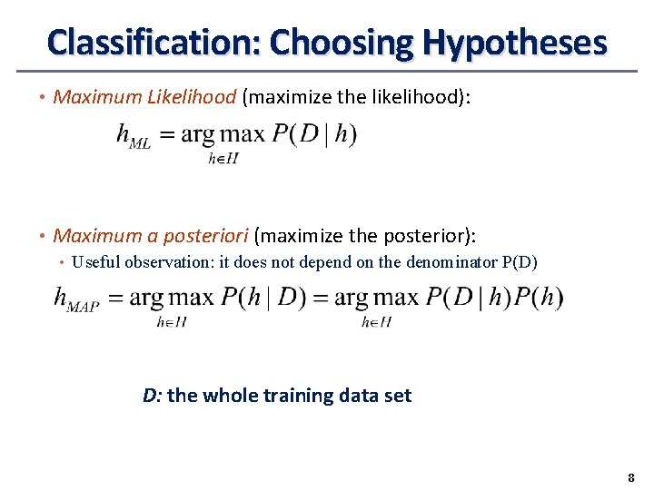
Classification: Choosing Hypotheses • Maximum Likelihood (maximize the likelihood): • Maximum a posteriori (maximize the posterior): • Useful observation: it does not depend on the denominator P(D) D: the whole training data set 8

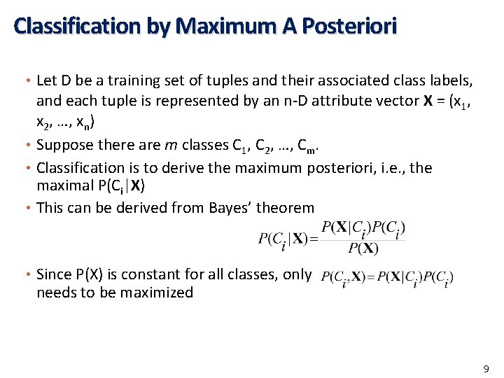
Classification by Maximum A Posteriori • Let D be a training set of tuples and their associated class labels, and each tuple is represented by an n-D attribute vector X = (x 1, x 2, …, xn) • Suppose there are m classes C 1, C 2, …, Cm. • Classification is to derive the maximum posteriori, i. e. , the maximal P(Ci|X) • This can be derived from Bayes’ theorem • Since P(X) is constant for all classes, only needs to be maximized 9

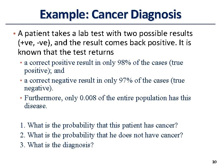
Example: Cancer Diagnosis • A patient takes a lab test with two possible results (+ve, -ve), and the result comes back positive. It is known that the test returns • a correct positive result in only 98% of the cases (true positive); and • a correct negative result in only 97% of the cases (true negative). • Furthermore, only 0. 008 of the entire population has this disease. 1. What is the probability that this patient has cancer? 2. What is the probability that he does not have cancer? 3. What is the diagnosis? 10

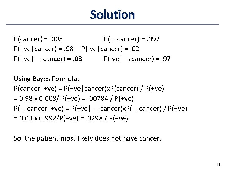
Solution P(cancer) =. 008 P( cancer) =. 992 P(+ve|cancer) =. 98 P(-ve|cancer) =. 02 P(+ve| cancer) =. 03 P(-ve| cancer) =. 97 Using Bayes Formula: P(cancer|+ve) = P(+ve|cancer)x. P(cancer) / P(+ve) = 0. 98 x 0. 008/ P(+ve) =. 00784 / P(+ve) P( cancer|+ve) = P(+ve| cancer)x. P( cancer) / P(+ve) = 0. 03 x 0. 992/P(+ve) =. 0298 / P(+ve) So, the patient most likely does not have cancer. 11

Chapter 8&9. Classification: Part 3 • Bayesian Learning • Naïve Bayes • Bayesian Belief Network • Instance-Based Learning • Summary 12

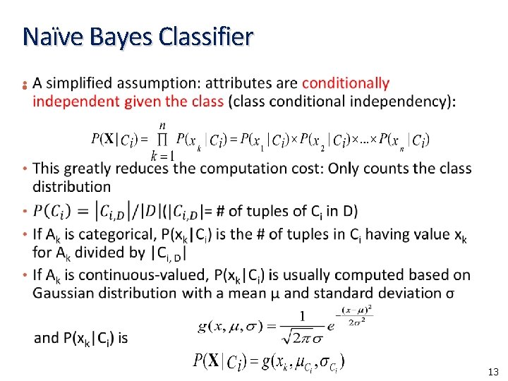
Naïve Bayes Classifier • 13

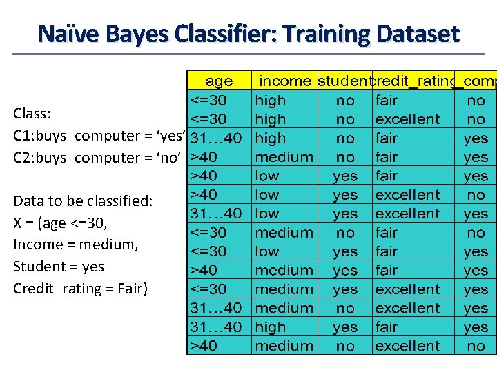
Naïve Bayes Classifier: Training Dataset Class: C 1: buys_computer = ‘yes’ C 2: buys_computer = ‘no’ Data to be classified: X = (age <=30, Income = medium, Student = yes Credit_rating = Fair)

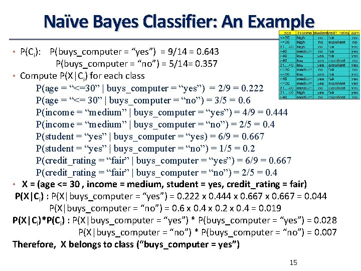
Naïve Bayes Classifier: An Example • P(Ci): P(buys_computer = “yes”) = 9/14 = 0. 643 P(buys_computer = “no”) = 5/14= 0. 357 • Compute P(X|Ci) for each class P(age = “<=30” | buys_computer = “yes”) = 2/9 = 0. 222 P(age = “<= 30” | buys_computer = “no”) = 3/5 = 0. 6 P(income = “medium” | buys_computer = “yes”) = 4/9 = 0. 444 P(income = “medium” | buys_computer = “no”) = 2/5 = 0. 4 P(student = “yes” | buys_computer = “yes) = 6/9 = 0. 667 P(student = “yes” | buys_computer = “no”) = 1/5 = 0. 2 P(credit_rating = “fair” | buys_computer = “yes”) = 6/9 = 0. 667 P(credit_rating = “fair” | buys_computer = “no”) = 2/5 = 0. 4 • X = (age <= 30 , income = medium, student = yes, credit_rating = fair) P(X|Ci) : P(X|buys_computer = “yes”) = 0. 222 x 0. 444 x 0. 667 = 0. 044 P(X|buys_computer = “no”) = 0. 6 x 0. 4 x 0. 2 x 0. 4 = 0. 019 P(X|Ci)*P(Ci) : P(X|buys_computer = “yes”) * P(buys_computer = “yes”) = 0. 028 P(X|buys_computer = “no”) * P(buys_computer = “no”) = 0. 007 Therefore, X belongs to class (“buys_computer = yes”) 15

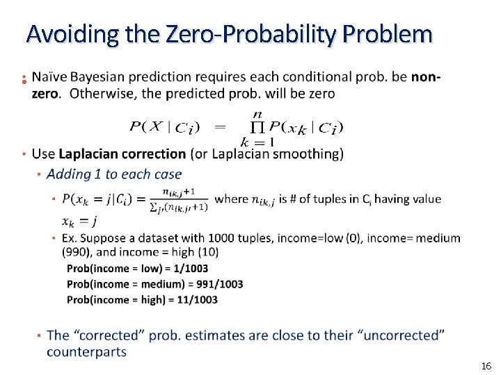
Avoiding the Zero-Probability Problem • 16

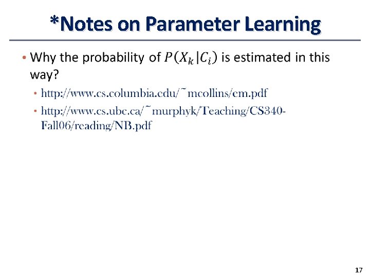
*Notes on Parameter Learning • 17

Naïve Bayes Classifier: Comments • Advantages • Easy to implement • Good results obtained in most of the cases • Disadvantages • Assumption: class conditional independence, therefore loss of accuracy • Practically, dependencies exist among variables • E. g. , hospitals: patients: Profile: age, family history, etc. Symptoms: fever, cough etc. , Disease: lung cancer, diabetes, etc. • Dependencies among these cannot be modeled by Naïve Bayes Classifier • How to deal with these dependencies? Bayesian Belief Networks 18

Chapter 8&9. Classification: Part 3 • Bayesian Learning • Naïve Bayes • Bayesian Belief Network • Instance-Based Learning • Summary 19

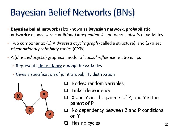
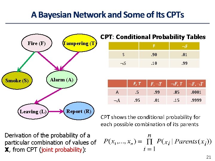
Bayesian Belief Networks (BNs) • Bayesian belief network (also known as Bayesian network, probabilistic network): allows class conditional independencies between subsets of variables • Two components: (1) A directed acyclic graph (called a structure) and (2) a set of conditional probability tables (CPTs) • A (directed acyclic) graphical model of causal influence relationships • Represents dependency among the variables • Gives a specification of joint probability distribution Y X Z P q Nodes: random variables q Links: dependency q X and Y are the parents of Z, and Y is the parent of P q No dependency between Z and P conditional on Y q Has no cycles 20

A Bayesian Network and Some of Its CPTs Fire (F) Tampering (T) CPT: Conditional Probability Tables F S Smoke (S) Alarm (A) Report (R) . 01 . 10 . 99 F, T A Leaving (L) . 90 . 5 . 99 . 85 . 0001 . 95 . 01 . 15 . 9999 CPT shows the conditional probability for each possible combination of its parents Derivation of the probability of a particular combination of values of X, from CPT (joint probability): 21

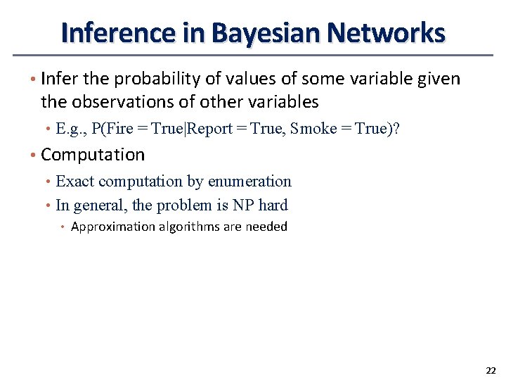
Inference in Bayesian Networks • Infer the probability of values of some variable given the observations of other variables • E. g. , P(Fire = True|Report = True, Smoke = True)? • Computation • Exact computation by enumeration • In general, the problem is NP hard • Approximation algorithms are needed 22

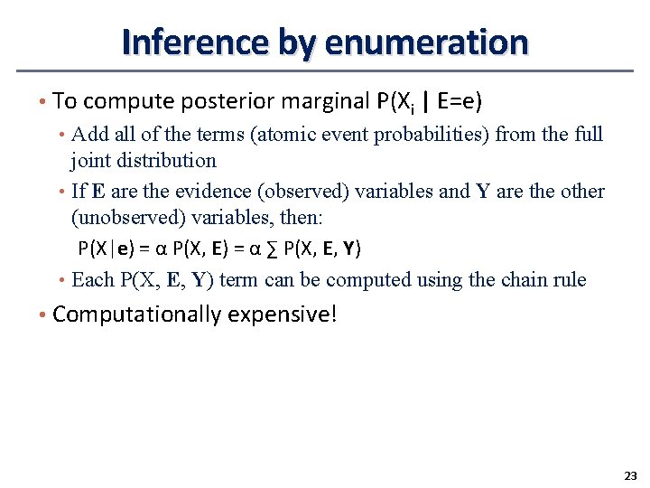
Inference by enumeration • To compute posterior marginal P(Xi | E=e) • Add all of the terms (atomic event probabilities) from the full joint distribution • If E are the evidence (observed) variables and Y are the other (unobserved) variables, then: P(X|e) = α P(X, E) = α ∑ P(X, E, Y) • Each P(X, E, Y) term can be computed using the chain rule • Computationally expensive! 23

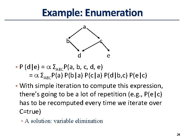
Example: Enumeration a b c d e • P (d|e) = ΣABCP(a, b, c, d, e) = ΣABCP(a) P(b|a) P(c|a) P(d|b, c) P(e|c) • With simple iteration to compute this expression, there’s going to be a lot of repetition (e. g. , P(e|c) has to be recomputed every time we iterate over C=true) • A solution: variable elimination 24

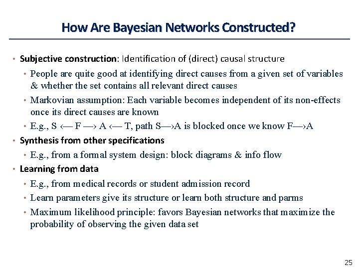
How Are Bayesian Networks Constructed? • Subjective construction: Identification of (direct) causal structure • People are quite good at identifying direct causes from a given set of variables & whether the set contains all relevant direct causes • Markovian assumption: Each variable becomes independent of its non-effects once its direct causes are known • E. g. , S ‹— F —› A ‹— T, path S—›A is blocked once we know F—›A • Synthesis from other specifications • E. g. , from a formal system design: block diagrams & info flow • Learning from data • E. g. , from medical records or student admission record • Learn parameters give its structure or learn both structure and parms • Maximum likelihood principle: favors Bayesian networks that maximize the probability of observing the given data set 25

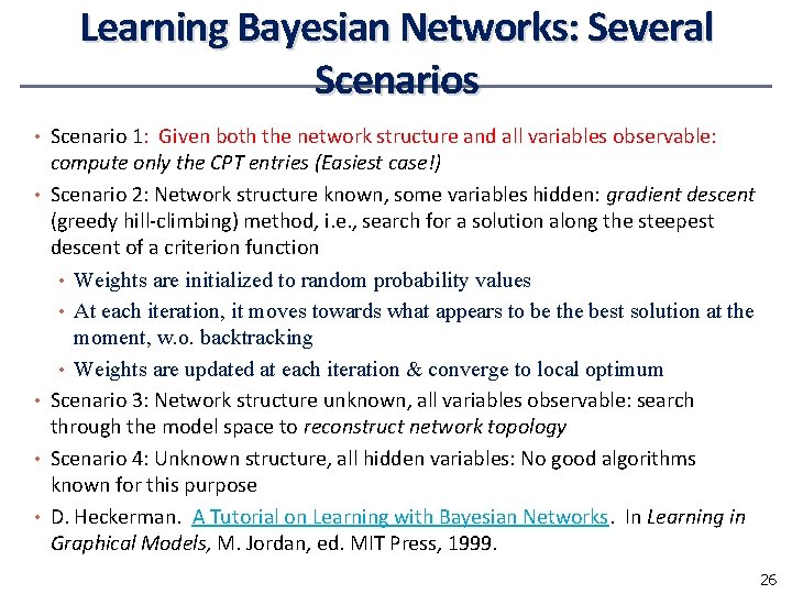
Learning Bayesian Networks: Several Scenarios • Scenario 1: Given both the network structure and all variables observable: • • compute only the CPT entries (Easiest case!) Scenario 2: Network structure known, some variables hidden: gradient descent (greedy hill-climbing) method, i. e. , search for a solution along the steepest descent of a criterion function • Weights are initialized to random probability values • At each iteration, it moves towards what appears to be the best solution at the moment, w. o. backtracking • Weights are updated at each iteration & converge to local optimum Scenario 3: Network structure unknown, all variables observable: search through the model space to reconstruct network topology Scenario 4: Unknown structure, all hidden variables: No good algorithms known for this purpose D. Heckerman. A Tutorial on Learning with Bayesian Networks. In Learning in Graphical Models, M. Jordan, ed. MIT Press, 1999. 26

Chapter 8&9. Classification: Part 3 • Bayesian Learning • Naïve Bayes • Bayesian Belief Network • Instance-Based Learning • Summary 27

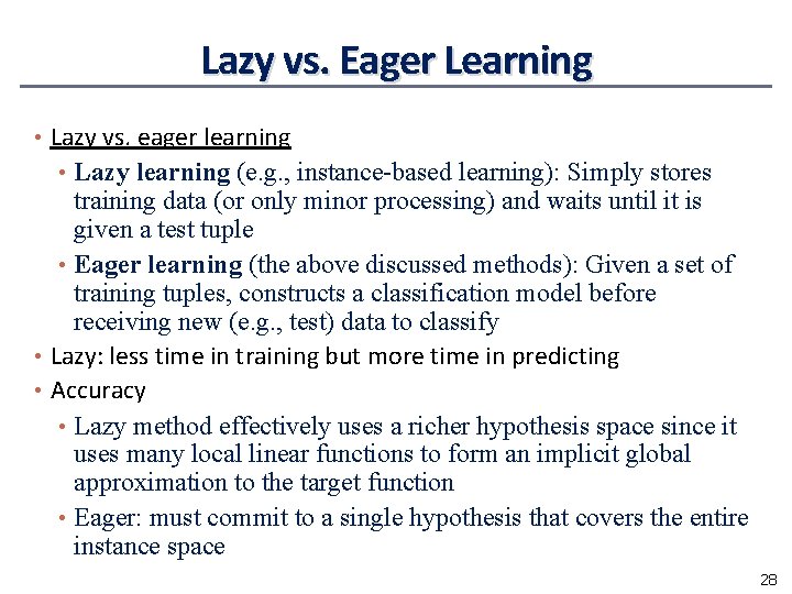
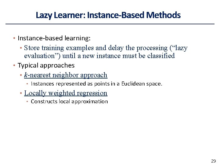
Lazy vs. Eager Learning • Lazy vs. eager learning • Lazy learning (e. g. , instance-based learning): Simply stores training data (or only minor processing) and waits until it is given a test tuple • Eager learning (the above discussed methods): Given a set of training tuples, constructs a classification model before receiving new (e. g. , test) data to classify • Lazy: less time in training but more time in predicting • Accuracy • Lazy method effectively uses a richer hypothesis space since it uses many local linear functions to form an implicit global approximation to the target function • Eager: must commit to a single hypothesis that covers the entire instance space 28

Lazy Learner: Instance-Based Methods • Instance-based learning: • Store training examples and delay the processing (“lazy evaluation”) until a new instance must be classified • Typical approaches • k-nearest neighbor approach • Instances represented as points in a Euclidean space. • Locally weighted regression • Constructs local approximation 29

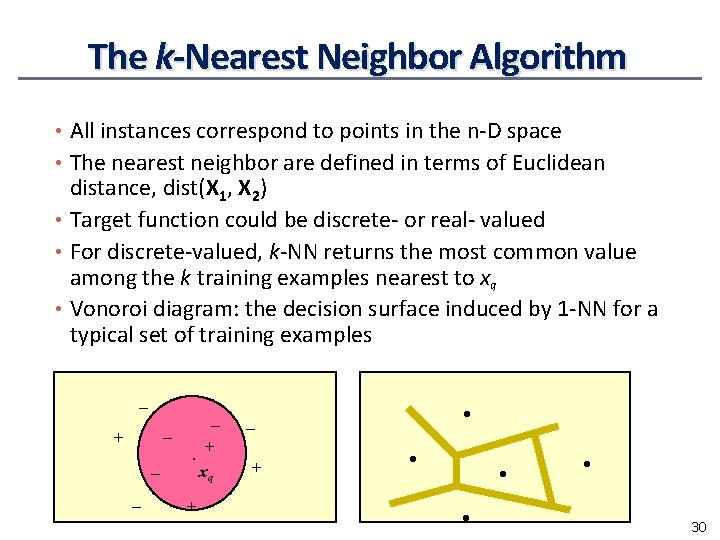
The k-Nearest Neighbor Algorithm • All instances correspond to points in the n-D space • The nearest neighbor are defined in terms of Euclidean distance, dist(X 1, X 2) • Target function could be discrete- or real- valued • For discrete-valued, k-NN returns the most common value among the k training examples nearest to xq • Vonoroi diagram: the decision surface induced by 1 -NN for a typical set of training examples _ _ + _ _ _. + xq + _ + . . . 30

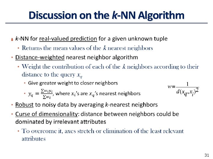
Discussion on the k-NN Algorithm • 31

Chapter 8&9. Classification: Part 3 • Bayesian Learning • Naïve Bayes • Bayesian Belief Network • Instance-Based Learning • Summary 32

Summary • Bayesian Learning • Bayes theorem • Naïve Bayes, class conditional independence • Bayesian Belief Network, DAG, conditional probability table • Instance-Based Learning • Lazy learning vs. eager learning • K-nearest neighbor algorithm 33