CS 5670 Computer Vision Feature matching Reading Szeliski

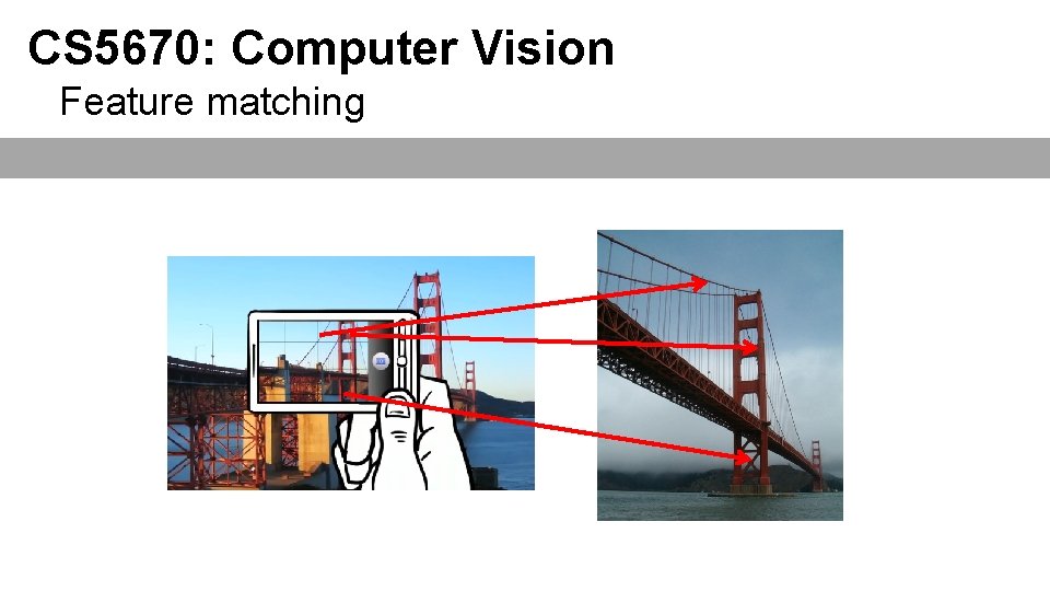
CS 5670: Computer Vision Feature matching

Reading • Szeliski (1 st edition): 4. 1

Announcements • Project 1 artifact due tonight at 11: 59 pm on CMSX • Project 2 out today, due Friday, March 12 at 7 pm – To be done in groups of two – will host breakout sessions at the end of class (last 10 minutes) • A (slightly shorter) quiz this Wednesday, due 7 minutes after the start of class

Project 2 Demo

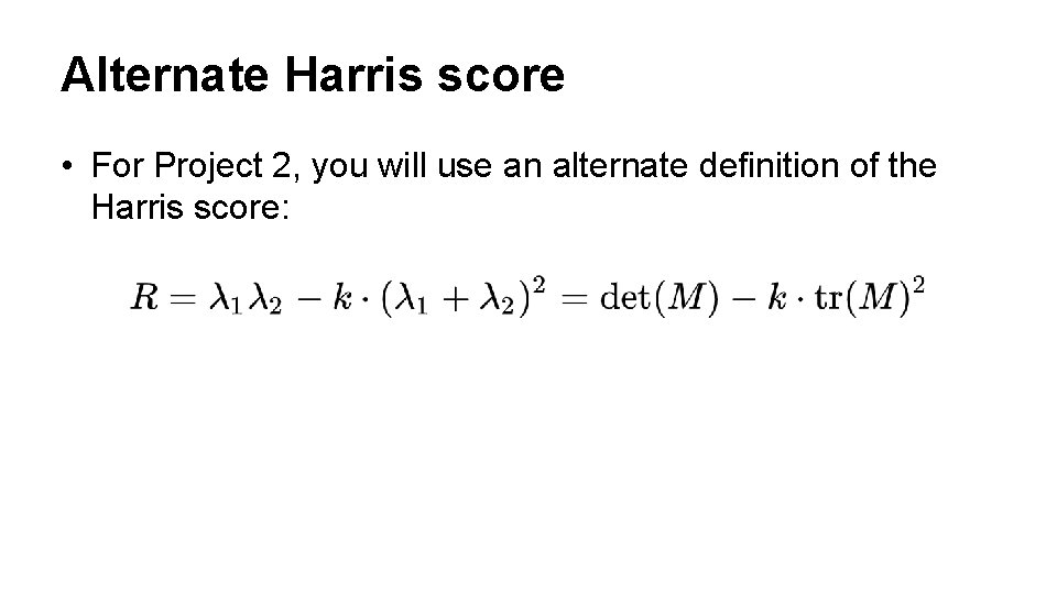
Alternate Harris score • For Project 2, you will use an alternate definition of the Harris score:

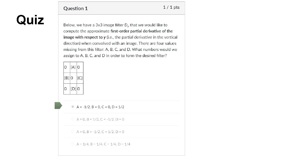
Quiz

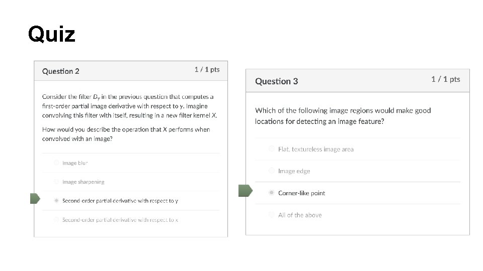
Quiz

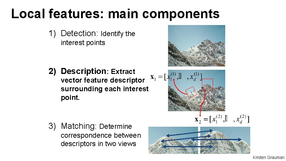
Local features: main components 1) Detection: Identify the interest points 2) Description: Extract vector feature descriptor surrounding each interest point. 3) Matching: Determine correspondence between descriptors in two views Kristen Grauman

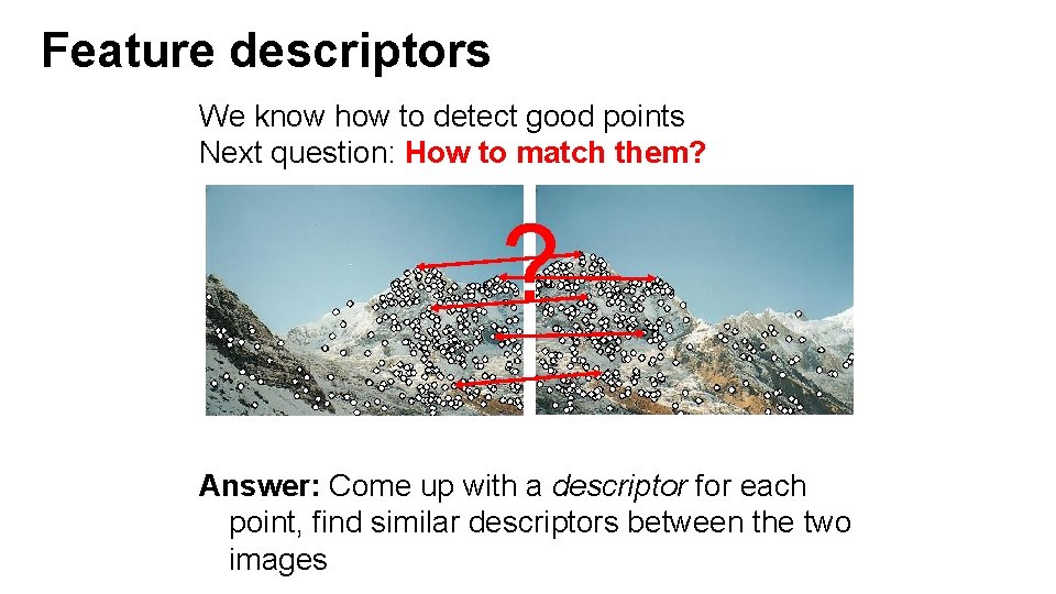
Feature descriptors We know how to detect good points Next question: How to match them? ? Answer: Come up with a descriptor for each point, find similar descriptors between the two images

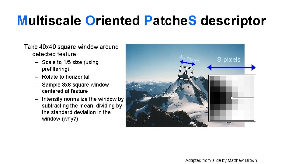
Multiscale Oriented Patche. S descriptor Take 40 x 40 square window around detected feature – Scale to 1/5 size (using prefiltering) – Rotate to horizontal – Sample 8 x 8 square window centered at feature – Intensity normalize the window by subtracting the mean, dividing by the standard deviation in the window (why? ) 40 pi xels 8 pixels CSE 576: Computer Vision Adapted from slide by Matthew Brown

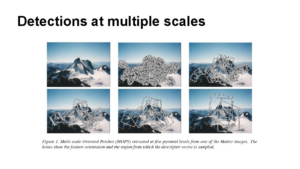
Detections at multiple scales

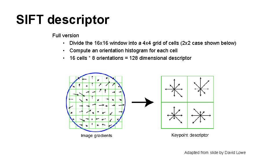
SIFT descriptor Full version • Divide the 16 x 16 window into a 4 x 4 grid of cells (2 x 2 case shown below) • Compute an orientation histogram for each cell • 16 cells * 8 orientations = 128 dimensional descriptor Adapted from slide by David Lowe

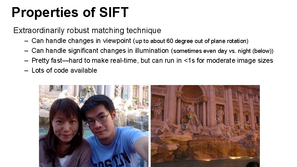
Properties of SIFT Extraordinarily robust matching technique – – Can handle changes in viewpoint (up to about 60 degree out of plane rotation) Can handle significant changes in illumination (sometimes even day vs. night (below)) Pretty fast—hard to make real-time, but can run in <1 s for moderate image sizes Lots of code available

Questions?

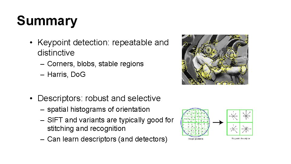
Summary • Keypoint detection: repeatable and distinctive – Corners, blobs, stable regions – Harris, Do. G • Descriptors: robust and selective – spatial histograms of orientation – SIFT and variants are typically good for stitching and recognition – Can learn descriptors (and detectors)

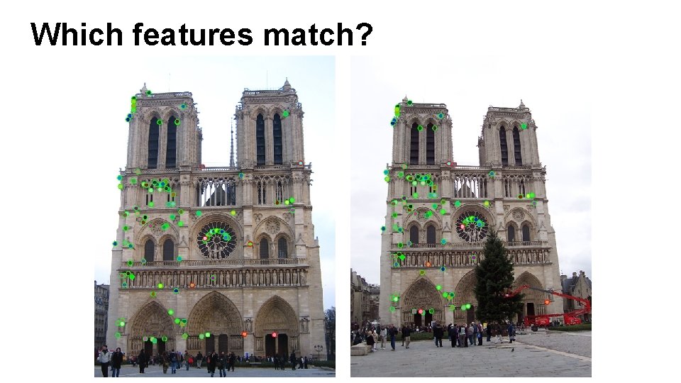
Which features match?

Feature matching Given a feature in I 1, how to find the best match in I 2? 1. Define distance function that compares two descriptors 2. Test all the features in I 2, find the one with min distance

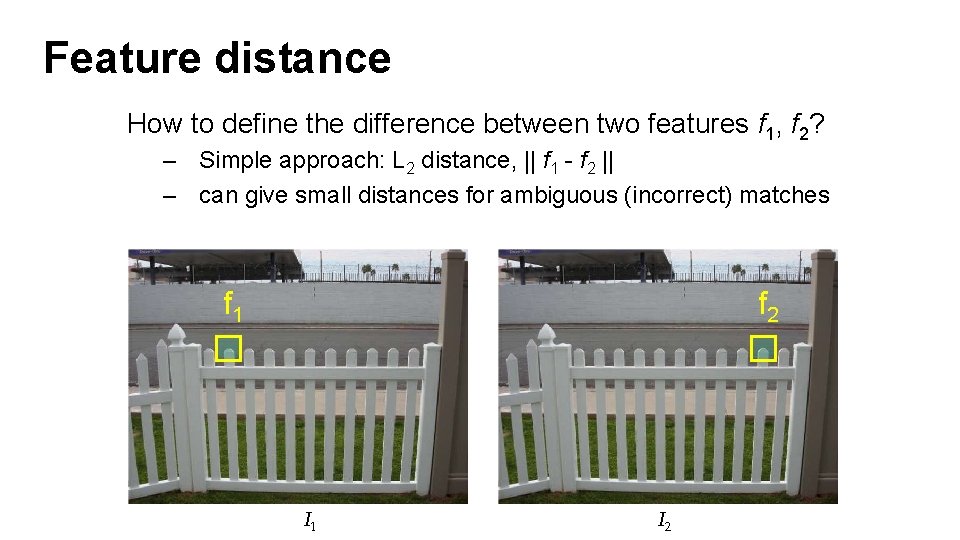
Feature distance How to define the difference between two features f 1, f 2? – Simple approach: L 2 distance, || f 1 - f 2 || – can give small distances for ambiguous (incorrect) matches f 1 f 2 I 1 I 2

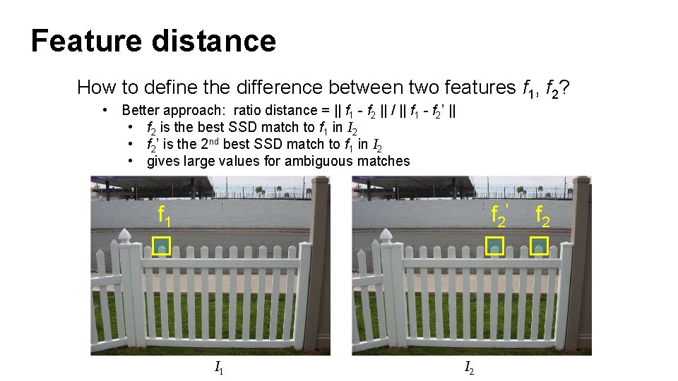
Feature distance How to define the difference between two features f 1, f 2? • Better approach: ratio distance = || f 1 - f 2 || / || f 1 - f 2’ || • f 2 is the best SSD match to f 1 in I 2 • f 2’ is the 2 nd best SSD match to f 1 in I 2 • gives large values for ambiguous matches f 1 f 2' I 1 I 2 f 2

Feature distance • Does the SSD vs “ratio distance” change the best match to a given feature in image 1?

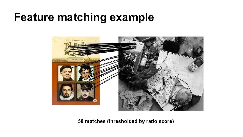
Feature matching example 58 matches (thresholded by ratio score)

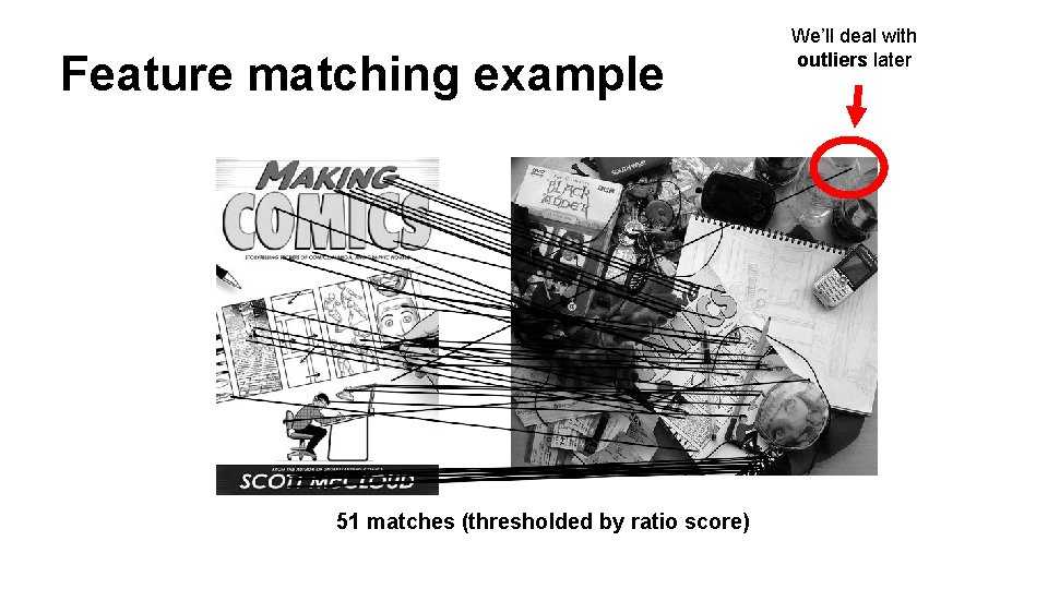
Feature matching example 51 matches (thresholded by ratio score) We’ll deal with outliers later

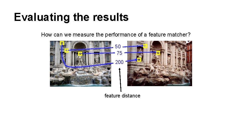
Evaluating the results How can we measure the performance of a feature matcher? 50 75 200 feature distance

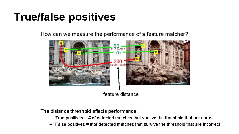
True/false positives How can we measure the performance of a feature matcher? 50 75 true match 200 false match feature distance The distance threshold affects performance – True positives = # of detected matches that survive threshold that are correct – False positives = # of detected matches that survive threshold that are incorrect

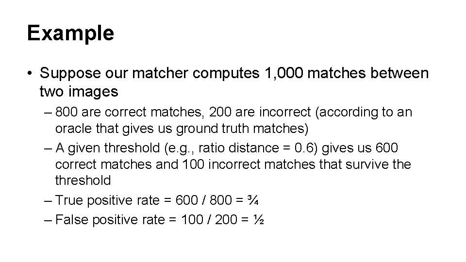
Example • Suppose our matcher computes 1, 000 matches between two images – 800 are correct matches, 200 are incorrect (according to an oracle that gives us ground truth matches) – A given threshold (e. g. , ratio distance = 0. 6) gives us 600 correct matches and 100 incorrect matches that survive threshold – True positive rate = 600 / 800 = ¾ – False positive rate = 100 / 200 = ½

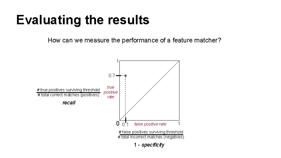
Evaluating the results How can we measure the performance of a feature matcher? 1 0. 7 true # true positives surviving threshold positive # total correct matches (positives) rate recall 0 0. 1 false positive rate 1 # false positives surviving threshold # total incorrect matches (negatives) 1 - specificity

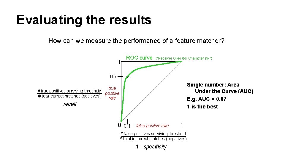
Evaluating the results How can we measure the performance of a feature matcher? 1 ROC curve (“Receiver Operator Characteristic”) 0. 7 Single number: Area Under the Curve (AUC) E. g. AUC = 0. 87 1 is the best true # true positives surviving threshold positive # total correct matches (positives) rate recall 0 0. 1 false positive rate 1 # false positives surviving threshold # total incorrect matches (negatives) 1 - specificity

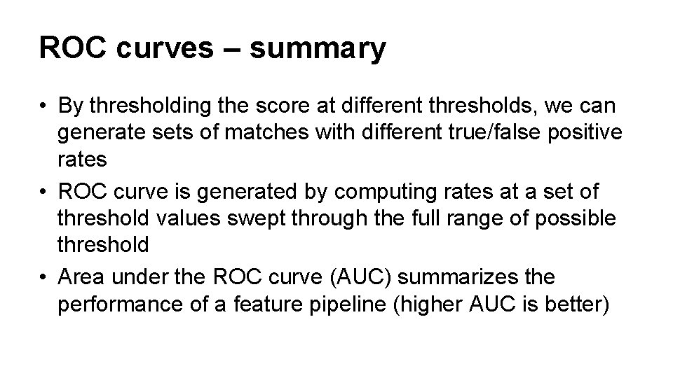
ROC curves – summary • By thresholding the score at different thresholds, we can generate sets of matches with different true/false positive rates • ROC curve is generated by computing rates at a set of threshold values swept through the full range of possible threshold • Area under the ROC curve (AUC) summarizes the performance of a feature pipeline (higher AUC is better)

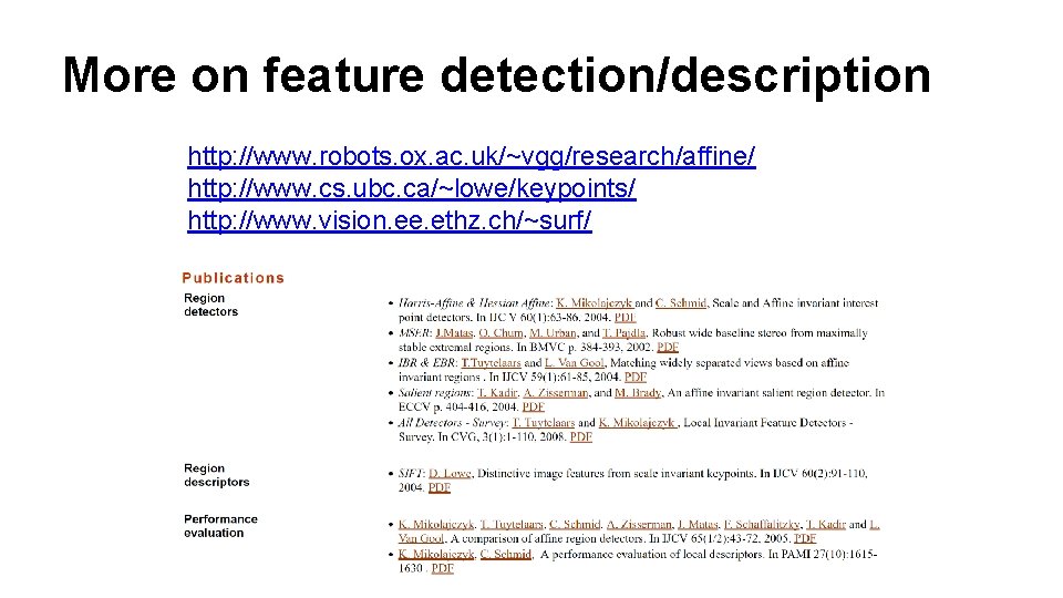
More on feature detection/description http: //www. robots. ox. ac. uk/~vgg/research/affine/ http: //www. cs. ubc. ca/~lowe/keypoints/ http: //www. vision. ee. ethz. ch/~surf/

Lots of applications Features are used for: – – – – Image alignment (e. g. , mosaics) 3 D reconstruction Motion tracking Object recognition Indexing and database retrieval Robot navigation … other

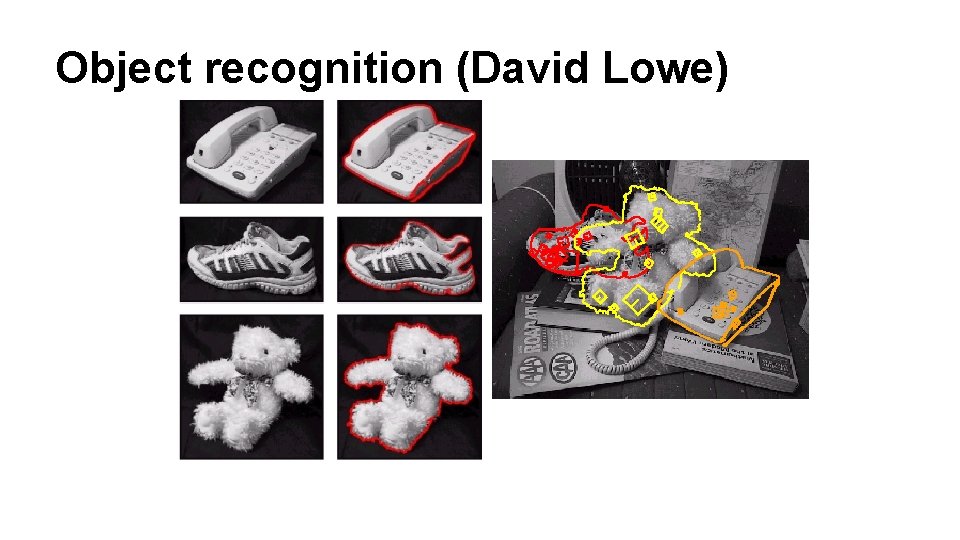
Object recognition (David Lowe)

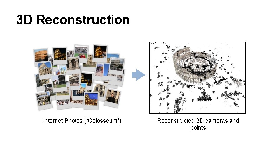
3 D Reconstruction Internet Photos (“Colosseum”) Reconstructed 3 D cameras and points

Augmented Reality

Live demo?

Questions?