CS 5670 Computer Vision Noah Snavely Lecture 5

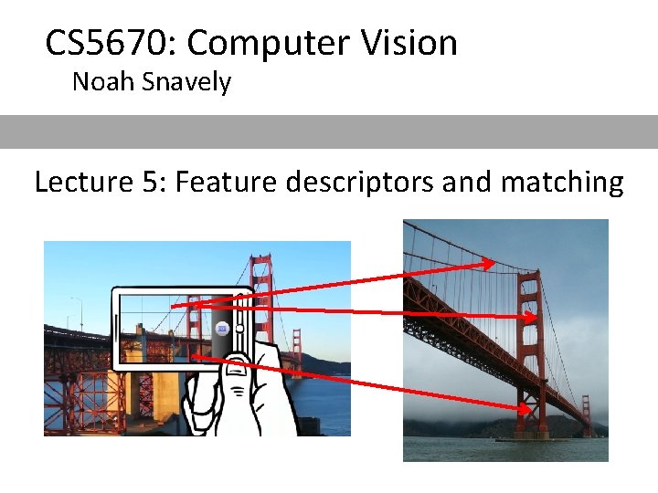
CS 5670: Computer Vision Noah Snavely Lecture 5: Feature descriptors and matching

Reading • Szeliski: 4. 1

Announcements • Project 2 is now released, due Monday, March 4, at 11: 59 pm – To be done in groups of 2 – Please create a group on CMS once you have found a partner • Project 1 artifact voting will be underway soon • Quiz 1 is graded and available on Gradescope

Project 2 Demo

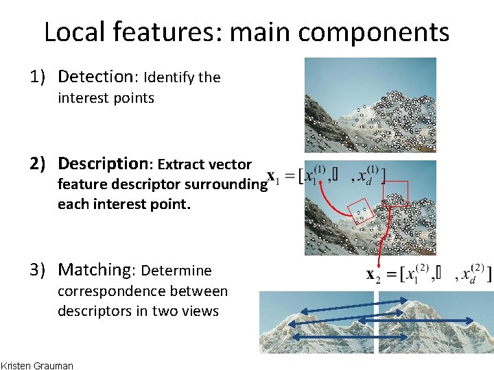
Local features: main components 1) Detection: Identify the interest points 2) Description: Extract vector feature descriptor surrounding each interest point. 3) Matching: Determine correspondence between descriptors in two views Kristen Grauman

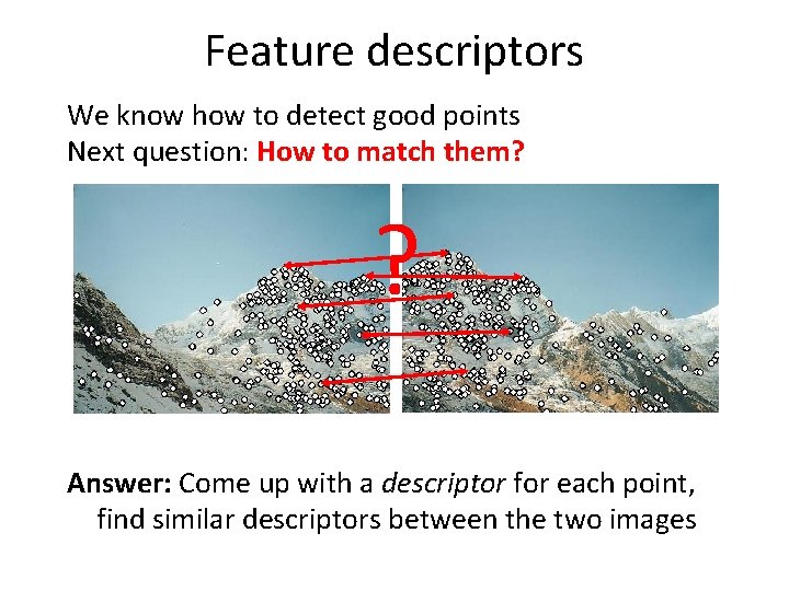
Feature descriptors We know how to detect good points Next question: How to match them? ? Answer: Come up with a descriptor for each point, find similar descriptors between the two images

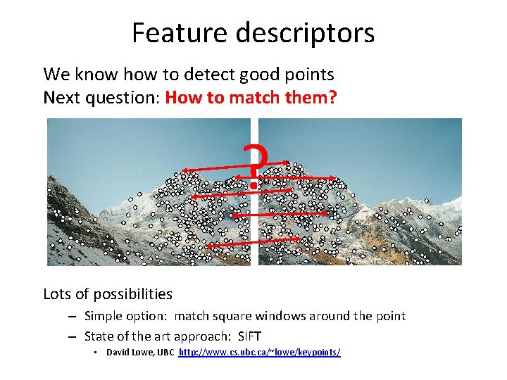
Feature descriptors We know how to detect good points Next question: How to match them? ? Lots of possibilities – Simple option: match square windows around the point – State of the art approach: SIFT • David Lowe, UBC http: //www. cs. ubc. ca/~lowe/keypoints/

Invariance vs. discriminability • Invariance: – Descriptor shouldn’t change even if image is transformed • Discriminability: – Descriptor should be highly unique for each point

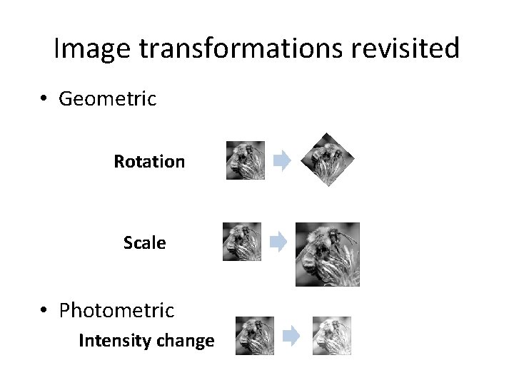
Image transformations revisited • Geometric Rotation Scale • Photometric Intensity change

Invariant descriptors • We looked at invariant / equivariant detectors • Most feature descriptors are also designed to be invariant to – Translation, 2 D rotation, scale • They can usually also handle – Limited 3 D rotations (SIFT works up to about 60 degrees) – Limited affine transforms (some are fully affine invariant) – Limited illumination/contrast changes

How to achieve invariance Need both of the following: 1. Make sure your detector is invariant 2. Design an invariant feature descriptor – Simplest descriptor: a single 0 • What’s this invariant to? – Next simplest descriptor: a square, axis-aligned 5 x 5 window of pixels • What’s this invariant to? – Let’s look at some better approaches…

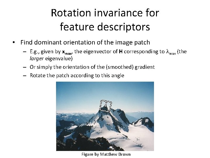
Rotation invariance for feature descriptors • Find dominant orientation of the image patch – E. g. , given by xmax, the eigenvector of H corresponding to max (the larger eigenvalue) – Or simply the orientation of the (smoothed) gradient – Rotate the patch according to this angle Figure by Matthew Brown

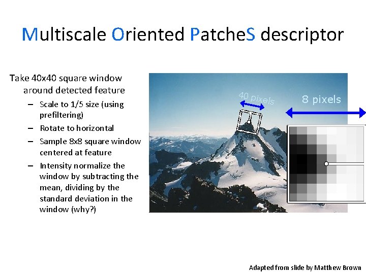
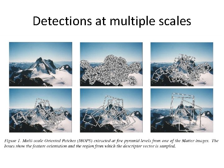
Multiscale Oriented Patche. S descriptor Take 40 x 40 square window around detected feature – Scale to 1/5 size (using prefiltering) – Rotate to horizontal – Sample 8 x 8 square window centered at feature – Intensity normalize the window by subtracting the mean, dividing by the standard deviation in the window (why? ) 40 pi xels 8 pixels CSE 576: Computer Vision Adapted from slide by Matthew Brown

Detections at multiple scales

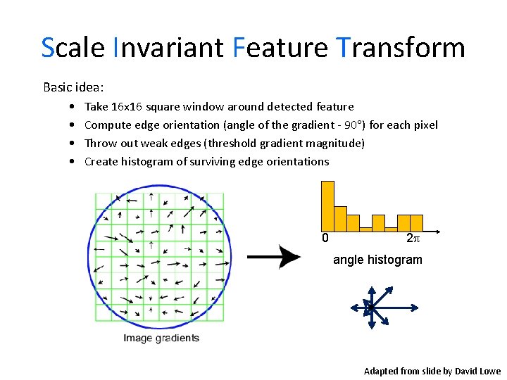
Scale Invariant Feature Transform Basic idea: • • Take 16 x 16 square window around detected feature Compute edge orientation (angle of the gradient - 90 ) for each pixel Throw out weak edges (threshold gradient magnitude) Create histogram of surviving edge orientations 0 2 angle histogram Adapted from slide by David Lowe

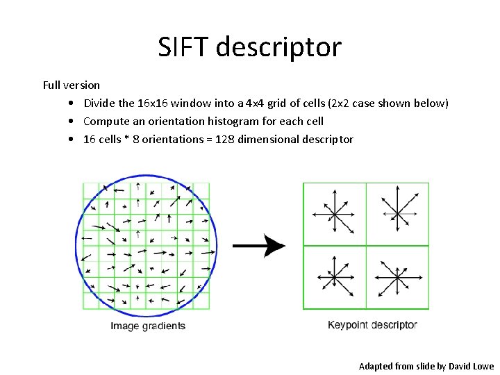
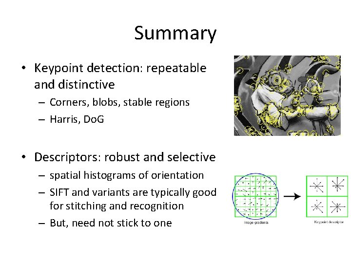
SIFT descriptor Full version • Divide the 16 x 16 window into a 4 x 4 grid of cells (2 x 2 case shown below) • Compute an orientation histogram for each cell • 16 cells * 8 orientations = 128 dimensional descriptor Adapted from slide by David Lowe

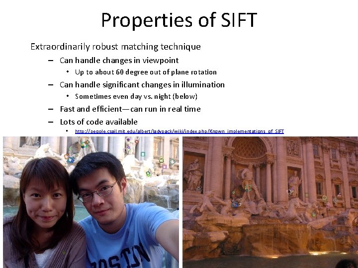
Properties of SIFT Extraordinarily robust matching technique – Can handle changes in viewpoint • Up to about 60 degree out of plane rotation – Can handle significant changes in illumination • Sometimes even day vs. night (below) – Fast and efficient—can run in real time – Lots of code available • http: //people. csail. mit. edu/albert/ladypack/wiki/index. php/Known_implementations_of_SIFT

SIFT Example sift 868 SIFT features

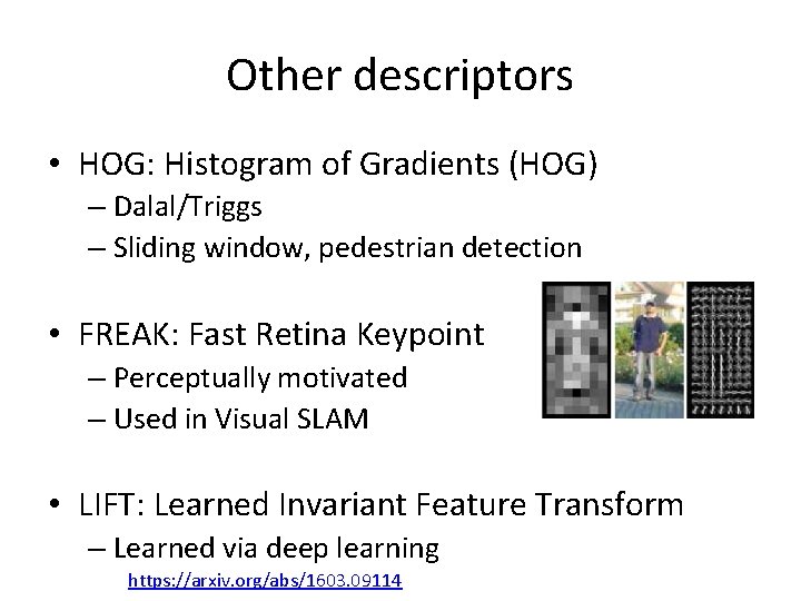
Other descriptors • HOG: Histogram of Gradients (HOG) – Dalal/Triggs – Sliding window, pedestrian detection • FREAK: Fast Retina Keypoint – Perceptually motivated – Used in Visual SLAM • LIFT: Learned Invariant Feature Transform – Learned via deep learning https: //arxiv. org/abs/1603. 09114

Questions?

Summary • Keypoint detection: repeatable and distinctive – Corners, blobs, stable regions – Harris, Do. G • Descriptors: robust and selective – spatial histograms of orientation – SIFT and variants are typically good for stitching and recognition – But, need not stick to one

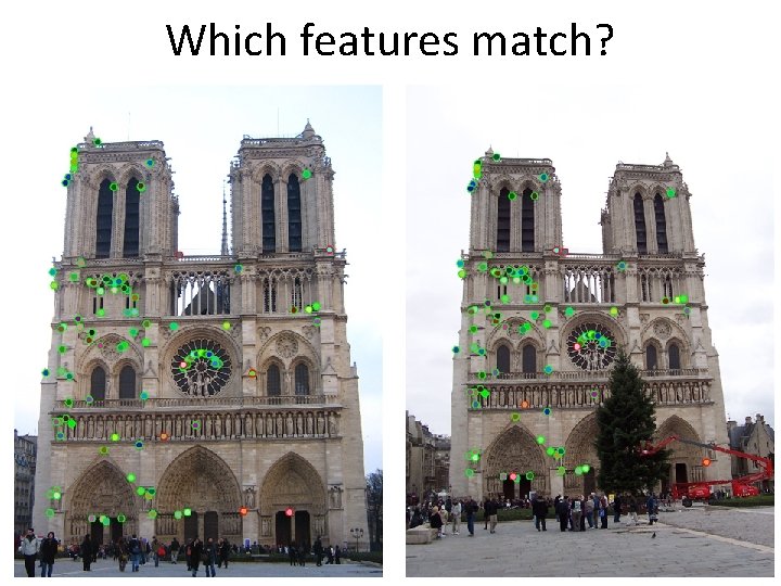
Which features match?

Feature matching Given a feature in I 1, how to find the best match in I 2? 1. Define distance function that compares two descriptors 2. Test all the features in I 2, find the one with min distance

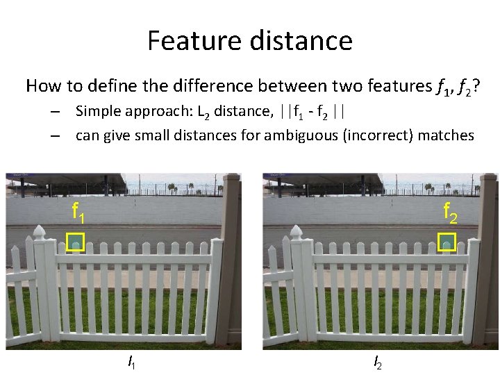
Feature distance How to define the difference between two features f 1, f 2? – Simple approach: L 2 distance, ||f 1 - f 2 || – can give small distances for ambiguous (incorrect) matches f 1 f 2 I 1 I 2

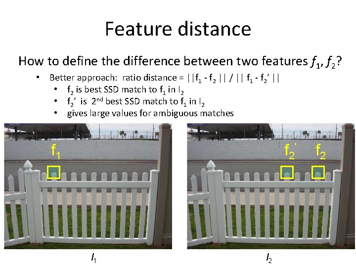
Feature distance How to define the difference between two features f 1, f 2? • Better approach: ratio distance = ||f 1 - f 2 || / || f 1 - f 2’ || • f 2 is best SSD match to f 1 in I 2 • f 2’ is 2 nd best SSD match to f 1 in I 2 • gives large values for ambiguous matches f 1 f 2' I 1 I 2 f 2

Feature distance • Does the SSD vs “ratio distance” change the best match to a given feature in image 1?

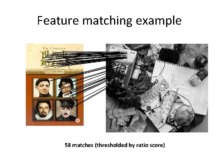
Feature matching example 58 matches (thresholded by ratio score)

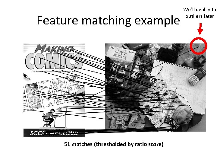
Feature matching example 51 matches (thresholded by ratio score) We’ll deal with outliers later

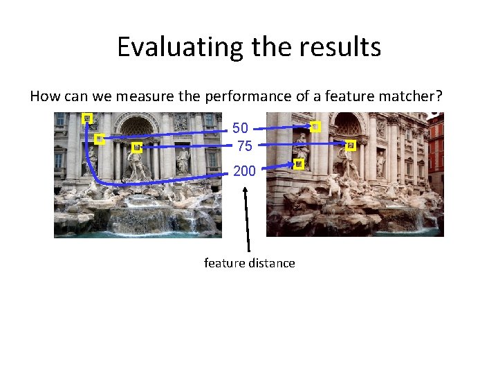
Evaluating the results How can we measure the performance of a feature matcher? 50 75 200 feature distance

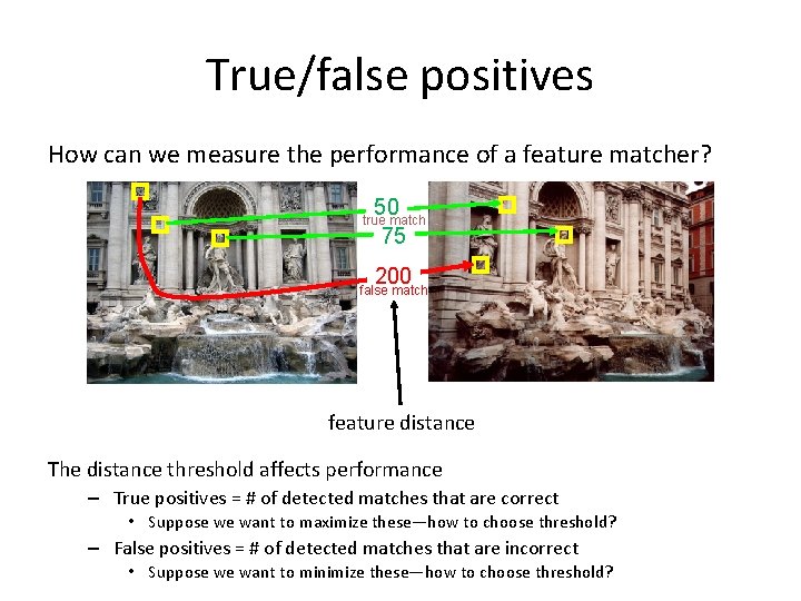
True/false positives How can we measure the performance of a feature matcher? 50 75 true match 200 false match feature distance The distance threshold affects performance – True positives = # of detected matches that are correct • Suppose we want to maximize these—how to choose threshold? – False positives = # of detected matches that are incorrect • Suppose we want to minimize these—how to choose threshold?

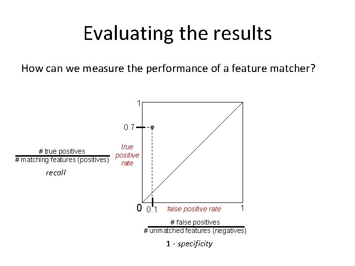
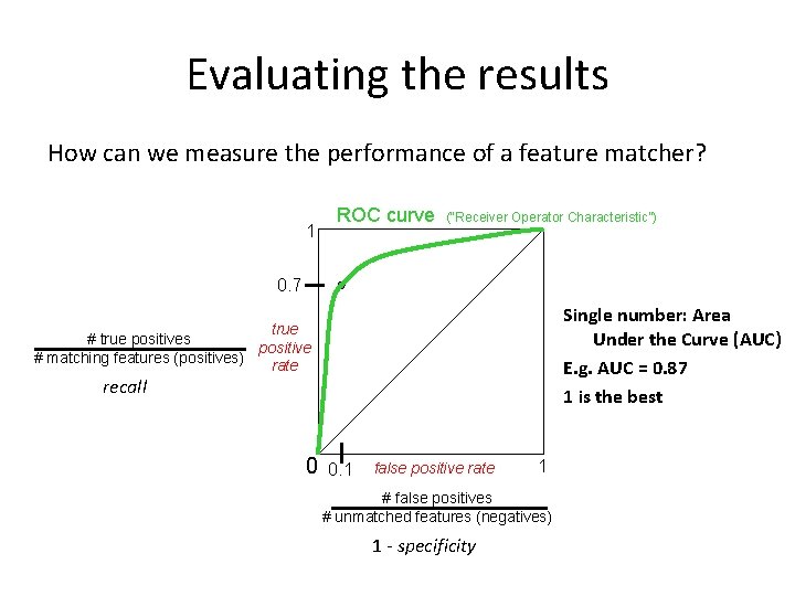
Evaluating the results How can we measure the performance of a feature matcher? 1 0. 7 true # true positives positive # matching features (positives) rate recall 0 0. 1 false positive rate 1 # false positives # unmatched features (negatives) 1 - specificity

Evaluating the results How can we measure the performance of a feature matcher? 1 ROC curve (“Receiver Operator Characteristic”) 0. 7 Single number: Area Under the Curve (AUC) E. g. AUC = 0. 87 1 is the best true # true positives positive # matching features (positives) rate recall 0 0. 1 false positive rate 1 # false positives # unmatched features (negatives) 1 - specificity

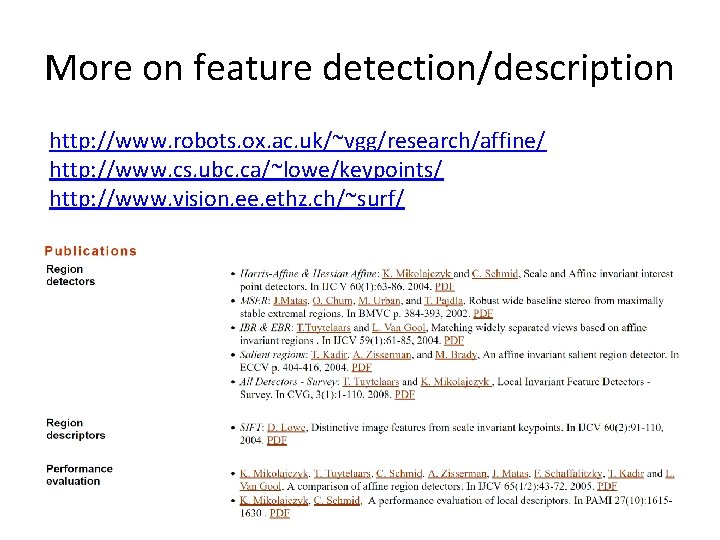
More on feature detection/description http: //www. robots. ox. ac. uk/~vgg/research/affine/ http: //www. cs. ubc. ca/~lowe/keypoints/ http: //www. vision. ee. ethz. ch/~surf/

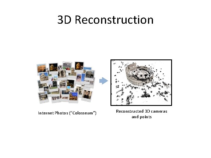
Lots of applications Features are used for: – – – – Image alignment (e. g. , mosaics) 3 D reconstruction Motion tracking Object recognition Indexing and database retrieval Robot navigation … other

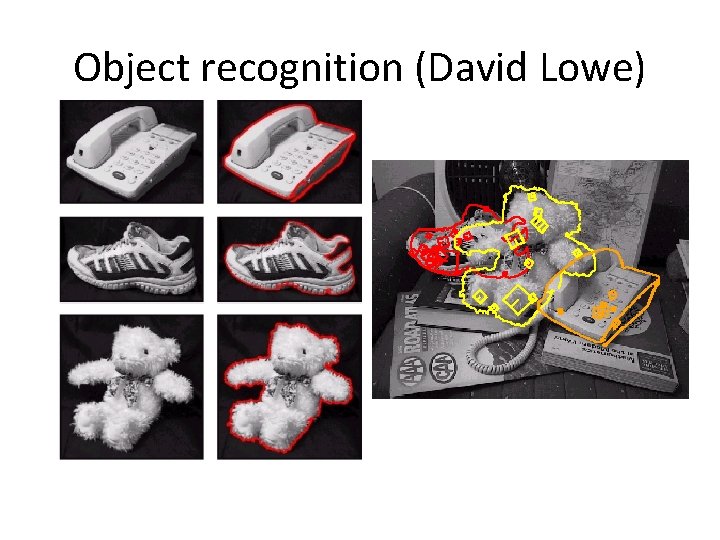
Object recognition (David Lowe)

3 D Reconstruction Internet Photos (“Colosseum”) Reconstructed 3 D cameras and points

Augmented Reality

Questions?