
CS 4670 5670 Computer Vision Noah Snavely Bagofwords
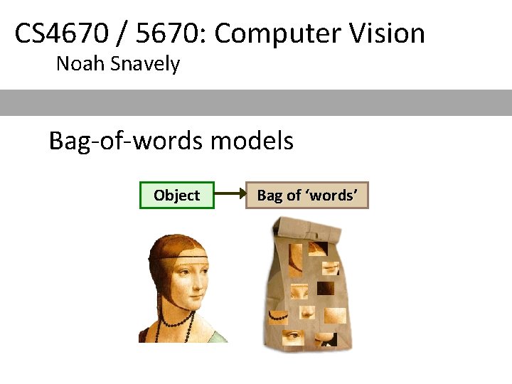
CS 4670 / 5670: Computer Vision Noah Snavely Bag-of-words models Object Bag of ‘words’
Bag of Words Models Adapted from slides by Rob Fergus and Svetlana Lazebnik
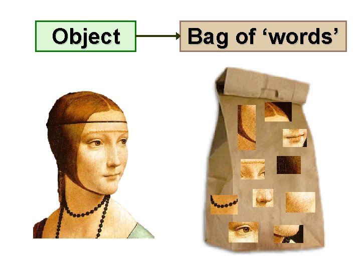
Object Bag of ‘words’
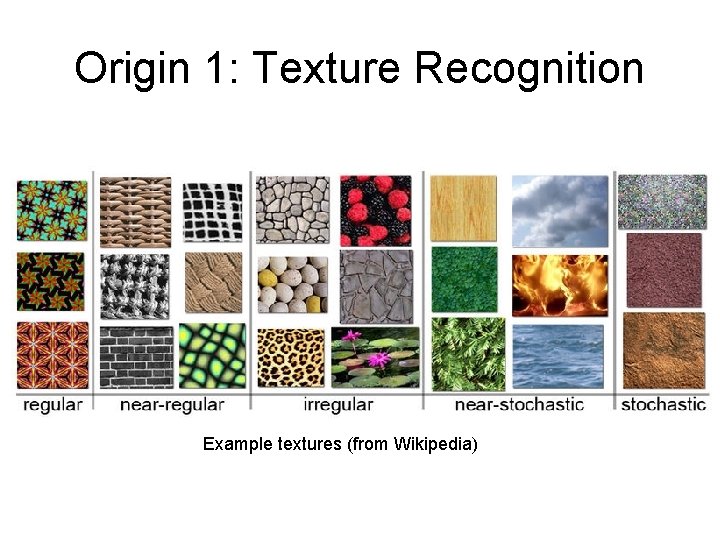
Origin 1: Texture Recognition Example textures (from Wikipedia)
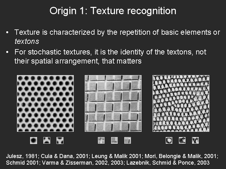
Origin 1: Texture recognition • Texture is characterized by the repetition of basic elements or textons • For stochastic textures, it is the identity of the textons, not their spatial arrangement, that matters Julesz, 1981; Cula & Dana, 2001; Leung & Malik 2001; Mori, Belongie & Malik, 2001; Schmid 2001; Varma & Zisserman, 2002, 2003; Lazebnik, Schmid & Ponce, 2003
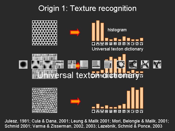
Origin 1: Texture recognition histogram Universal texton dictionary Julesz, 1981; Cula & Dana, 2001; Leung & Malik 2001; Mori, Belongie & Malik, 2001; Schmid 2001; Varma & Zisserman, 2002, 2003; Lazebnik, Schmid & Ponce, 2003
Origin 2: Bag-of-words models • Orderless document representation: frequencies of words from a dictionary Salton & Mc. Gill (1983)
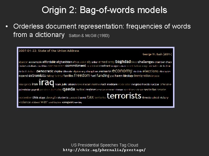
Origin 2: Bag-of-words models • Orderless document representation: frequencies of words from a dictionary Salton & Mc. Gill (1983) US Presidential Speeches Tag Cloud http: //chir. ag/phernalia/preztags/
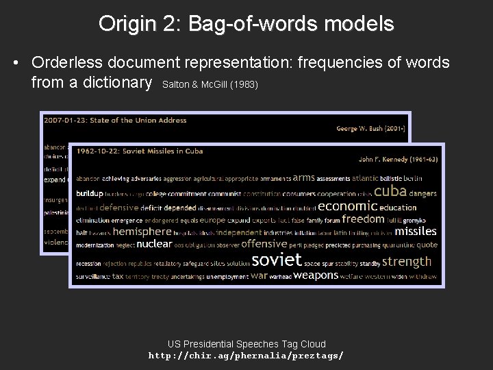
Origin 2: Bag-of-words models • Orderless document representation: frequencies of words from a dictionary Salton & Mc. Gill (1983) US Presidential Speeches Tag Cloud http: //chir. ag/phernalia/preztags/
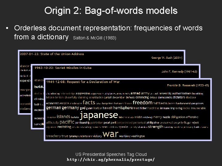
Origin 2: Bag-of-words models • Orderless document representation: frequencies of words from a dictionary Salton & Mc. Gill (1983) US Presidential Speeches Tag Cloud http: //chir. ag/phernalia/preztags/
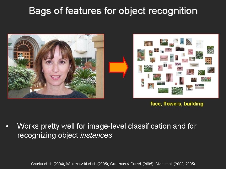
Bags of features for object recognition face, flowers, building • Works pretty well for image-level classification and for recognizing object instances Csurka et al. (2004), Willamowski et al. (2005), Grauman & Darrell (2005), Sivic et al. (2003, 2005)
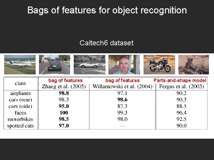
Bags of features for object recognition Caltech 6 dataset bag of features Parts-and-shape model
Bag of features • First, take a bunch of images, extract features, and build up a “dictionary” or “visual vocabulary” – a list of common features • Given a new image, extract features and build a histogram – for each feature, find the closest visual word in the dictionary
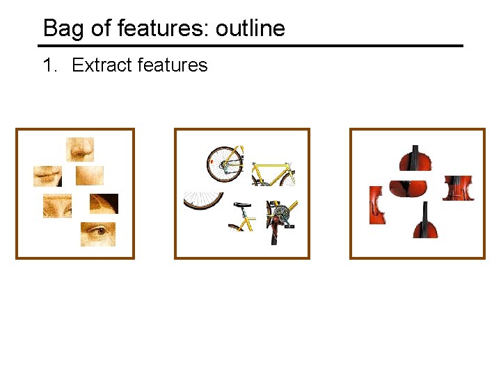
Bag of features: outline 1. Extract features
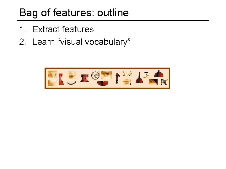
Bag of features: outline 1. Extract features 2. Learn “visual vocabulary”
Bag of features: outline 1. Extract features 2. Learn “visual vocabulary” 3. Quantize features using visual vocabulary
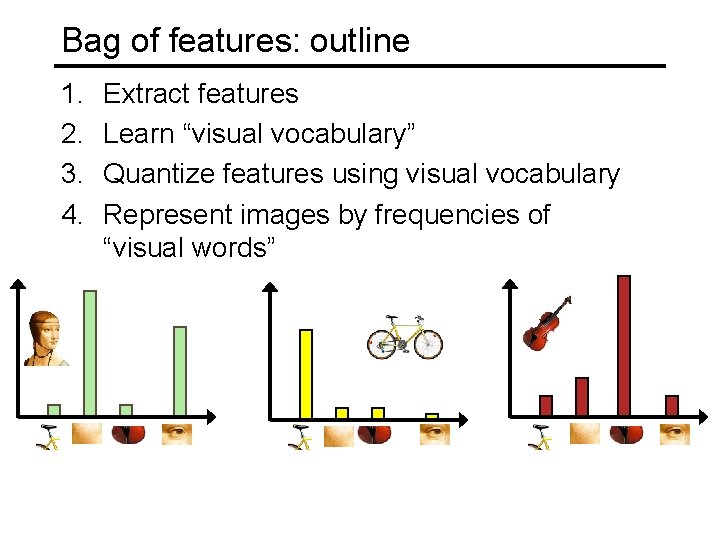
Bag of features: outline 1. 2. 3. 4. Extract features Learn “visual vocabulary” Quantize features using visual vocabulary Represent images by frequencies of “visual words”
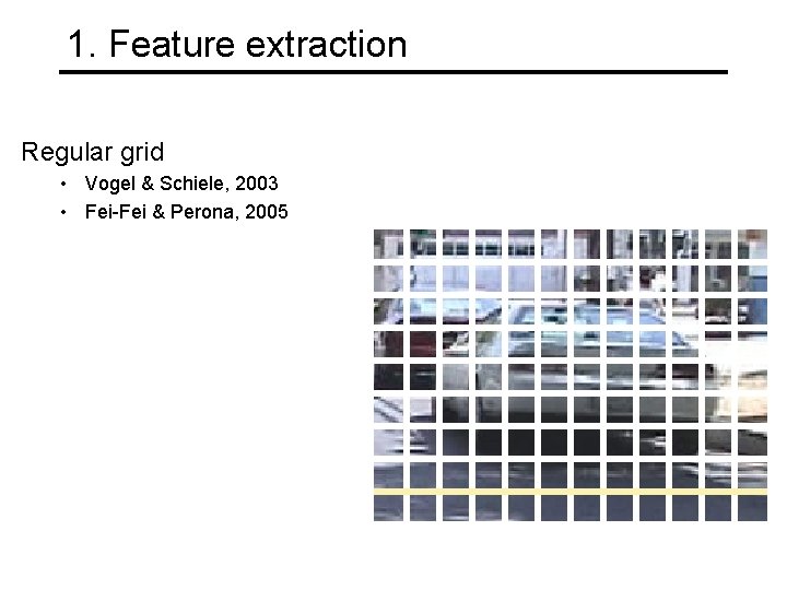
1. Feature extraction Regular grid • Vogel & Schiele, 2003 • Fei-Fei & Perona, 2005
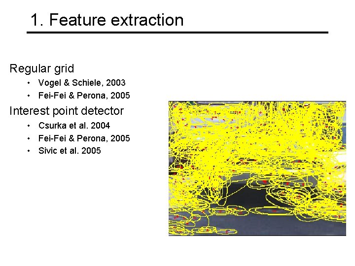
1. Feature extraction Regular grid • Vogel & Schiele, 2003 • Fei-Fei & Perona, 2005 Interest point detector • Csurka et al. 2004 • Fei-Fei & Perona, 2005 • Sivic et al. 2005
1. Feature extraction Regular grid • Vogel & Schiele, 2003 • Fei-Fei & Perona, 2005 Interest point detector • Csurka et al. 2004 • Fei-Fei & Perona, 2005 • Sivic et al. 2005 Other methods • Random sampling (Vidal-Naquet & Ullman, 2002) • Segmentation-based patches (Barnard et al. 2003)
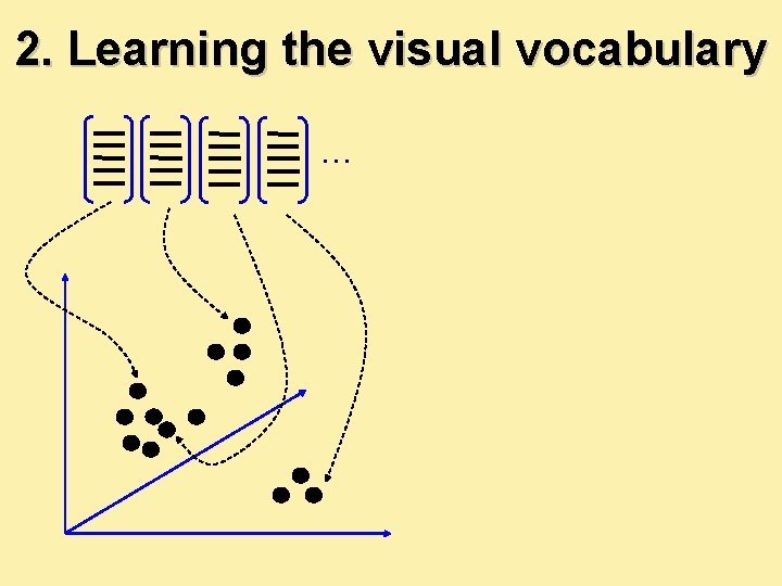
2. Learning the visual vocabulary …
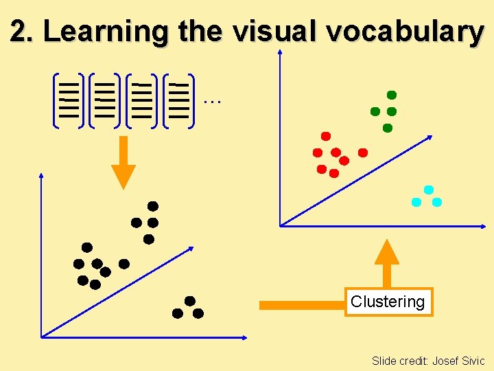
2. Learning the visual vocabulary … Clustering Slide credit: Josef Sivic
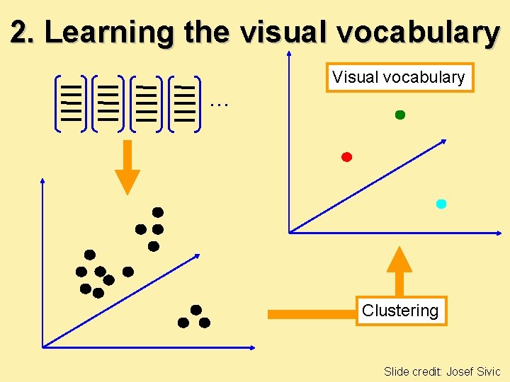
2. Learning the visual vocabulary … Visual vocabulary Clustering Slide credit: Josef Sivic
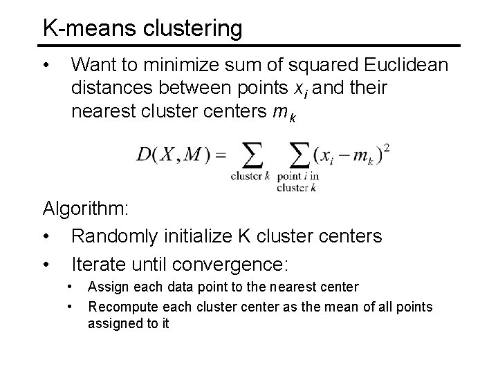
K-means clustering • Want to minimize sum of squared Euclidean distances between points xi and their nearest cluster centers mk Algorithm: • Randomly initialize K cluster centers • Iterate until convergence: • • Assign each data point to the nearest center Recompute each cluster center as the mean of all points assigned to it
From clustering to vector quantization • Clustering is a common method for learning a visual vocabulary or codebook • Unsupervised learning process • Each cluster center produced by k-means becomes a codevector • Codebook can be learned on separate training set • Provided the training set is sufficiently representative, the codebook will be “universal” • The codebook is used for quantizing features • A vector quantizer takes a feature vector and maps it to the index of the nearest codevector in a codebook • Codebook = visual vocabulary • Codevector = visual word
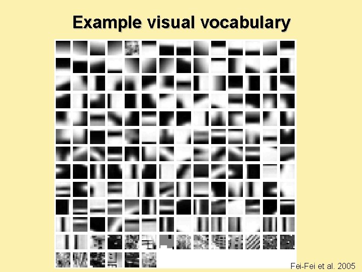
Example visual vocabulary Fei-Fei et al. 2005
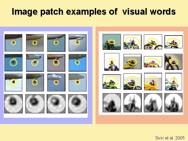
Image patch examples of visual words Sivic et al. 2005
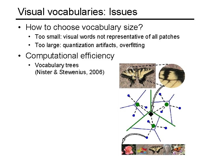
Visual vocabularies: Issues • How to choose vocabulary size? • Too small: visual words not representative of all patches • Too large: quantization artifacts, overfitting • Computational efficiency • Vocabulary trees (Nister & Stewenius, 2006)
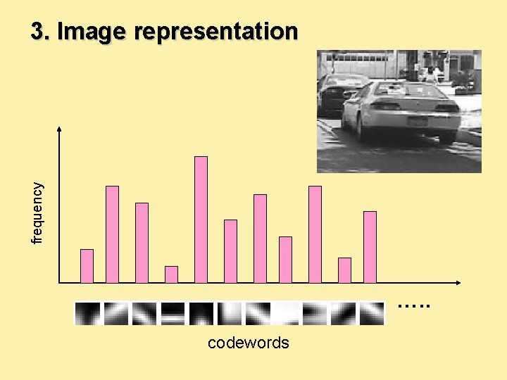
frequency 3. Image representation …. . codewords
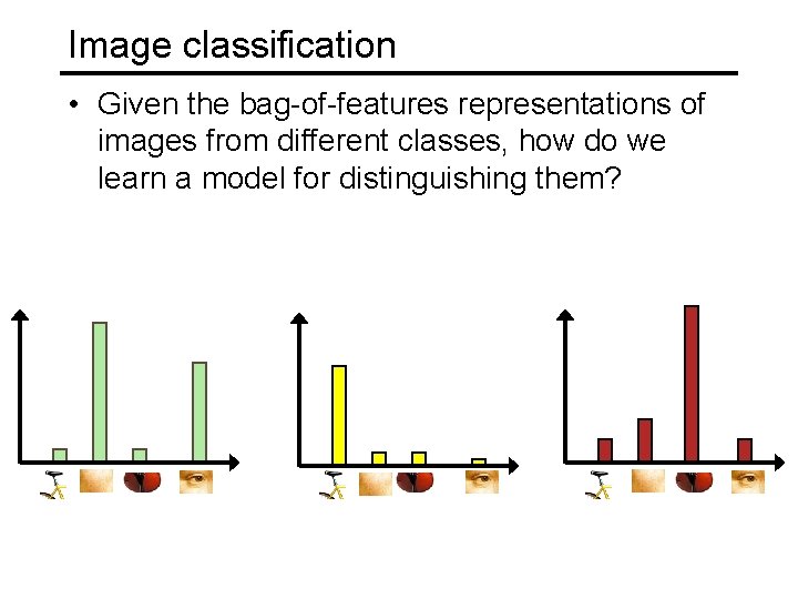
Image classification • Given the bag-of-features representations of images from different classes, how do we learn a model for distinguishing them?
Uses of Bo. W representation • Treat as feature vector for standard classifier – e. g k-nearest neighbors, support vector machine • Cluster Bo. W vectors over image collection – Discover visual themes
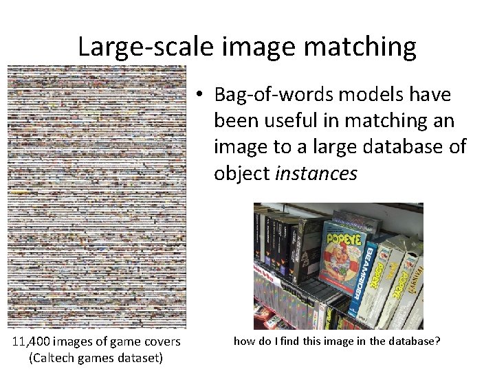
Large-scale image matching • Bag-of-words models have been useful in matching an image to a large database of object instances 11, 400 images of game covers (Caltech games dataset) how do I find this image in the database?
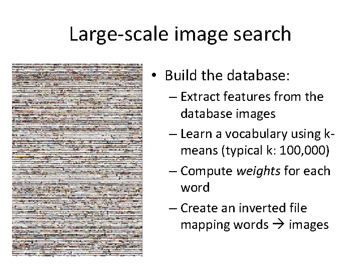
Large-scale image search • Build the database: – Extract features from the database images – Learn a vocabulary using kmeans (typical k: 100, 000) – Compute weights for each word – Create an inverted file mapping words images
Weighting the words • Just as with text, some visual words are more discriminative than others the, and, or vs. cow, AT&T, Cher • the bigger fraction of the documents a word appears in, the less useful it is for matching – e. g. , a word that appears in all documents is not helping us
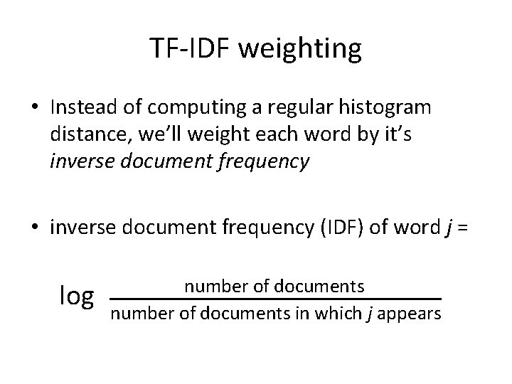
TF-IDF weighting • Instead of computing a regular histogram distance, we’ll weight each word by it’s inverse document frequency • inverse document frequency (IDF) of word j = log number of documents in which j appears
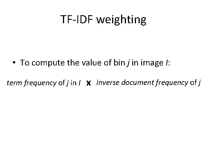
TF-IDF weighting • To compute the value of bin j in image I: term frequency of j in I x inverse document frequency of j
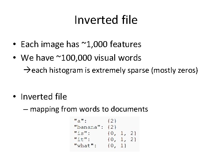
Inverted file • Each image has ~1, 000 features • We have ~100, 000 visual words each histogram is extremely sparse (mostly zeros) • Inverted file – mapping from words to documents
Inverted file • Can quickly use the inverted file to compute similarity between a new image and all the images in the database – Only consider database images whose bins overlap the query image
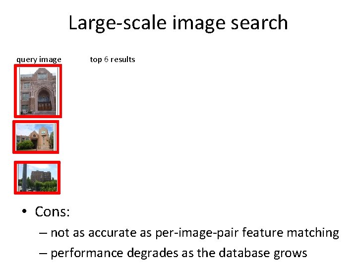
Large-scale image search query image top 6 results • Cons: – not as accurate as per-image-pair feature matching – performance degrades as the database grows
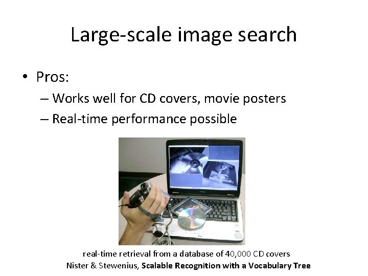
Large-scale image search • Pros: – Works well for CD covers, movie posters – Real-time performance possible real-time retrieval from a database of 40, 000 CD covers Nister & Stewenius, Scalable Recognition with a Vocabulary Tree
Large-scale image matching Turn 1, 000 images of Rome…
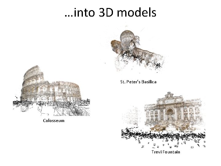
…into 3 D models St. Peter’s Basilica Colosseum Trevi Fountain
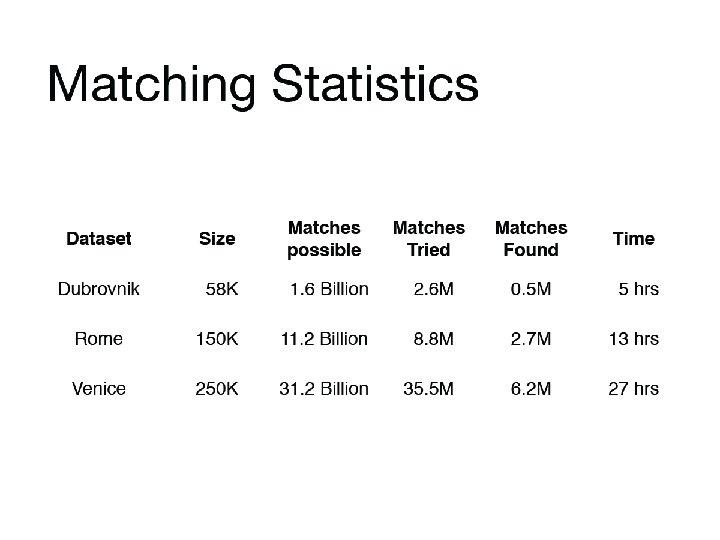
Large-scale image matching • How can we match 1, 000 images to each other? • Brute force approach: 500, 000, 000 pairs – won’t scale • Better approach: use bag-of-words technique to find likely matches • For each image, find the top M scoring other images, do detailed SIFT matching with those
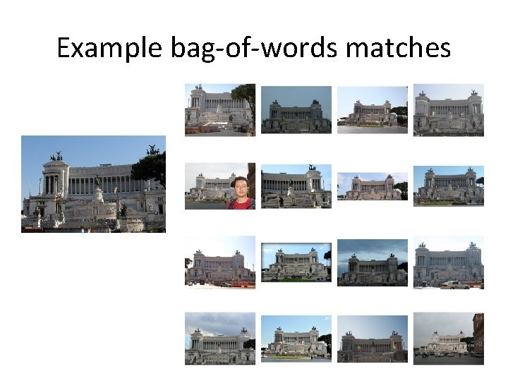
Example bag-of-words matches
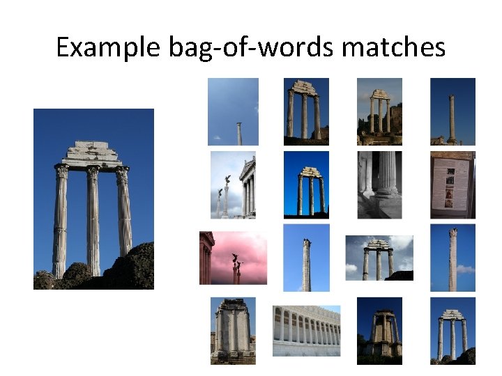
Example bag-of-words matches
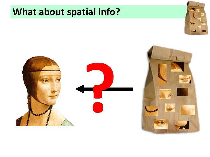
What about spatial info? ?
- Slides: 47