CSE 185 Introduction to Computer Vision Feature Matching

CSE 185 Introduction to Computer Vision Feature Matching

Feature matching • Keypoint matching • Hough transform • Reading: Chapter 4

Feature matching • Correspondence: matching points, patches, edges, or regions across images ≈

Keypoint matching B 3 A 1 A 2 A 3 B 2 B 1 1. Find a set of distinctive keypoints 2. Define a region around each keypoint 3. Extract and normalize the region content 4. Compute a local descriptor from the normalized region 5. Match local descriptors

Review: Interest points • Keypoint detection: repeatable and distinctive – Corners, blobs, stable regions – Harris, Do. G, MSER – SIFT

Which interest detector • What do you want it for? – Precise localization in x-y: Harris – Good localization in scale: Difference of Gaussian – Flexible region shape: MSER • Best choice often application dependent – Harris-/Hessian-Laplace/Do. G work well for many natural categories – MSER works well for buildings and printed things • Why choose? – Get more points with more detectors • There have been extensive evaluations/comparisons – [Mikolajczyk et al. , IJCV’ 05, PAMI’ 05] – All detectors/descriptors shown here work well

Local feature descriptors • Most features can be thought of as templates, histograms (counts), or combinations • The ideal descriptor should be – Robust and distinctive – Compact and efficient • Most available descriptors focus on edge/gradient information – Capture texture information – Color rarely used • Scale-invariant feature transform (SIFT) descriptor

How to decide which features match?

Feature matching • Szeliski 4. 1. 3 – Simple feature-space methods – Evaluation methods – Acceleration methods – Geometric verification (Chapter 6)

Feature matching • Simple criteria: One feature matches to another if those features are nearest neighbors and their distance is below some threshold. • Problems: – Threshold is difficult to set – Non-distinctive features could have lots of close matches, only one of which is correct

Matching local features • Threshold based on the ratio of 1 st nearest neighbor to 2 nd nearest neighbor distance Reject all matches in which the distance ration > 0. 8, which eliminates 90% of false matches while discarding less than 5% correct matches

SIFT repeatability It shows the stability of detection for keypoint location, orientation, and final matching to a database as a function of affine distortion. The degree of affine distortion is expressed in terms of the equivalent viewpoint rotation in depth for a planar surface.

Matching features What do we do about the “bad” matches? Blue line: randomly selected line Red line: outlier

RAndom SAmple Consensus Select one match, count inliers Blue line: randomly selected line Red line: outlier

RAndom SAmple Consensus Select one match, count inliers Blue line: randomly selected line Red line: outlier

Least squares fit Find “average” translation vector Blue line: randomly selected line Red line: outlier

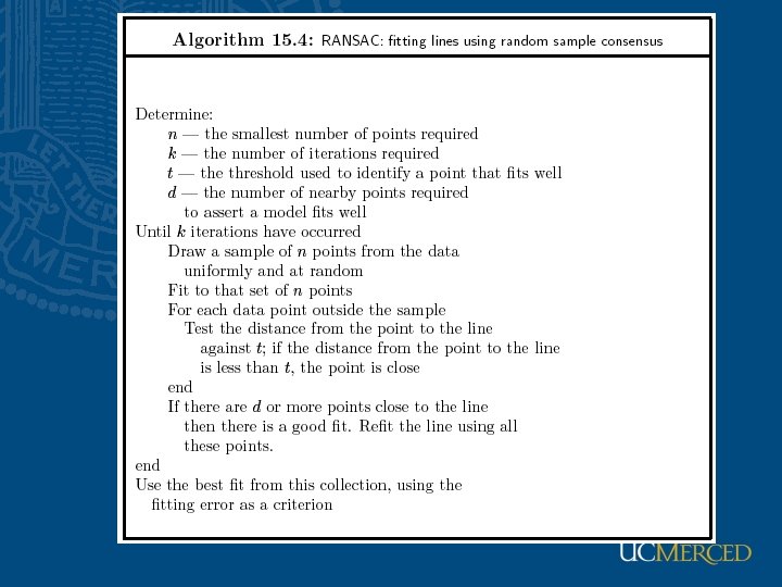
RANSAC • Random Sample Consensus • Choose a small subset uniformly at random • Fit to that • Anything that is close to result is signal; all others are noise • Refit • Do this many times and choose the best • Issues – How many times? • Often enough that we are likely to have a good line – How big a subset? • Smallest possible – What does close mean? • Depends on the problem – What is a good line? • One where the number of nearby points is so big it is unlikely to be all outliers

Descriptor Vector • Orientation = blurred gradient • Similarity Invariant Frame – Scale-space position (x, y, s) + orientation ( ) Image Stitching 19

RANSAC for Homography • SIFT features of two similar images

RANSAC for Homography • SIFT features common to both images

RANSAC for Homography • Select random subset of features (e. g. 6) • Compute motion estimate • Apply motion estimate to all SIFT features • Compute error: feature pairs not described by motion estimate • Repeat many times (e. g. 500) • Keep estimate with best error

RANSAC for Homography

Probabilistic model for verification • Potential problem: • Two images don’t match… • … but RANSAC found a motion estimate • Do a quick check to make sure the images do match • MAP for inliers vs. outliers

Finding the panoramas

Finding the panoramas Finding connected components

Finding the panoramas

Results

Fitting and alignment Fitting: find the parameters of a model that best fit the data Alignment: find the parameters of the transformation that best align matched points

Checkerboard • Often used in camera calibration See https: //docs. opencv. org/master/d 9/dab/tutorial_homography. html https: //www. mathworks. com/help/vision/ref/estimatecameraparameters. html

Fitting and alignment • Design challenges – Design a suitable goodness of fit measure • Similarity should reflect application goals • Encode robustness to outliers and noise – Design an optimization method • Avoid local optima • Find best parameters quickly

Fitting and alignment: Methods • Global optimization / Search for parameters – Least squares fit – Robust least squares – Iterative closest point (ICP) • Hypothesize and test – Generalized Hough transform – RANSAC

Least squares line fitting • Data: (x 1, y 1), …, (xn, yn) • Line equation: yi = m xi + b • Find (m, b) to minimize y=mx+b (xi, yi) Matlab: p = A y;

Least squares (global) optimization Good • Clearly specified objective • Optimization is easy Bad • May not be what you want to optimize • Sensitive to outliers – Bad matches, extra points • Doesn’t allow you to get multiple good fits – Detecting multiple objects, lines, etc.

Hypothesize and test 1. Propose parameters – – – Try all possible Each point votes for all consistent parameters Repeatedly sample enough points to solve for parameters 2. Score the given parameters – Number of consistent points, possibly weighted by distance 3. Choose from among the set of parameters – Global or local maximum of scores 4. Possibly refine parameters using inliers

Hough transform: Outline 1. Create a grid of parameter values 2. Each point votes for a set of parameters, incrementing those values in grid 3. Find maximum or local maxima in grid

Hough transform Given a set of points, find the curve or line that explains the data points best y Duality: Each point has a dual line in the parameter space m x y=mx+b m and b are known variables y and x are unknown variables Hough space b m = -(1/x)b + y/x x and y are known variables m and b are unknown variables

Hough transform y m b x y m 3 x 5 3 3 2 2 3 7 11 10 4 3 2 1 1 0 5 3 2 3 4 1 b

Hough transform Issue : parameter space [m, b] is unbounded… Use a polar representation for the parameter space Duality: Each point has a dual curve in the parameter space y x Hough space

Hough transform: Experiments features votes

Hough transform

Hough transform: Experiments Noisy data features Need to adjust grid size or smooth votes

Hough transform: Experiments features votes Issue: spurious peaks due to uniform noise

1. Image Canny

2. Canny Hough votes

3. Hough votes Edges Find peaks and post-process

Hough transform example

Hough transform: Finding lines • Using m, b parameterization • Using r, theta parameterization – Using oriented gradients • Practical considerations – Bin size – Smoothing – Finding multiple lines – Finding line segments