CS 46705670 Computer Vision Kavita Bala Lecture 13

CS 4670/5670: Computer Vision Kavita Bala Lecture 13: Feature Descriptors and Matching

Announcements • PA 2 out • Artifact voting out: please vote • Schedule will be updated shortly • HW 1 out tonight – No slip days for HW 1 – Due on Sunday Mar 13, answers released on Monday

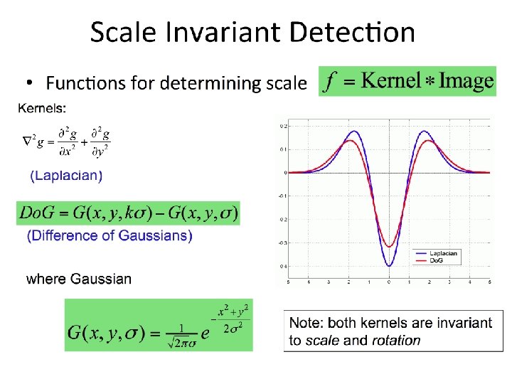
Another type of feature • The Laplacian of Gaussian (Lo. G) (very similar to a Difference of Gaussians (Do. G) – i. e. a Gaussian minus a slightly smaller Gaussian)

Comparison of Keypoint Detectors Tuytelaars Mikolajczyk 2008

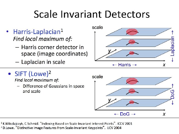
Choosing a detector • What do you want it for? – Precise localization in x-y: Harris – Good localization in scale: Difference of Gaussian – Flexible region shape: e. g. , Maximal Stable Extremal Regions • Best choice often application dependent • There have been extensive evaluations/comparisons – [Mikolajczyk et al. , IJCV’ 05, PAMI’ 05] – All detectors/descriptors shown here work well

Feature descriptors We know how to detect good points Next question: How to match them? ? Answer: Come up with a descriptor for each point, find similar descriptors between the two images

Feature descriptors We know how to detect good points Next question: How to match them? ? Lots of possibilities (this is a popular research area) – Simple option: match square windows around the point – State of the art approach: SIFT • David Lowe, UBC http: //www. cs. ubc. ca/~lowe/keypoints/

Image representations • Templates – Intensity, gradients, etc. • Histograms – Color, texture, SIFT descriptors, etc.

Local Descriptors • Most features can be thought of as templates, histograms (counts), or combinations • The ideal descriptor should be – Robust – Distinctive – Compact – Efficient • Most available descriptors focus on edge/gradient information – Capture texture information K. Grauman, B. Leibe

Image Representations: Histograms Global histogram • Represent distribution of features – Color, texture, depth, … Images from Dave Kauchak Space Shuttle Cargo Bay

What kind of things do we compute histograms of? • Color L*a*b* color space HSV color space • Texture (filter banks or HOG over regions) – HOG: Histogram of Oriented Gradients

Orientation Normalization [Lowe, SIFT, 1999] • Compute orientation histogram • Select dominant orientation • Normalize: rotate to fixed orientation 0 T. Tuytelaars, B. Leibe 2

Rotation invariance for feature descriptors • Find dominant orientation of the image patch – This is given by xmax, the eigenvector of M corresponding to max (the larger eigenvalue) – Rotate the patch according to this angle Figure by Matthew Brown

Multiscale Oriented Patche. S descriptor Take 40 x 40 square window around detected feature – Scale to 1/5 size (using prefiltering) – Rotate to horizontal – Sample 8 x 8 square window centered at feature – Intensity normalize the window by subtracting the mean, dividing by the standard deviation in the window 40 pi xels 8 pixels CSE 576: Computer Vision Adapted from slide by Matthew Brown

MOPS descriptor • You can combine transformations together to get the final transformation x T=? y

Translate x y T = MT 1

Rotate x y T = MRMT 1

Scale x y T = MSMRMT 1

Translate x y T = MT 2 MSMRMT 1

Crop x y

Detections at multiple scales

Invariance of MOPS • Intensity • Scale • Rotation

What kind of things do we compute histograms of? SIFT – Lowe IJCV 2004

Scale Invariant Feature Transform Basic idea: • Do. G for scale-space feature detection • Take 16 x 16 square window around detected feature • Compute gradient orientation for each pixel • Throw out weak edges (threshold gradient magnitude) • Create histogram of surviving edge orientations 0 2 angle histogram Adapted from slide by David Lowe

SIFT descriptor Create histogram • Divide the 16 x 16 window into a 4 x 4 grid of cells (2 x 2 case shown below) • Compute an orientation histogram for each cell • 16 cells * 8 orientations = 128 dimensional descriptor Adapted from slide by David Lowe

SIFT vector formation • Computed on rotated and scaled version of window according to computed orientation & scale – resample the window • Based on gradients weighted by a Gaussian

Ensure smoothness • Trilinear interpolation – a given gradient contributes to 8 bins: 4 in space times 2 in orientation

Reduce effect of illumination • 128 -dim vector normalized to 1 • Threshold gradient magnitudes to avoid excessive influence of high gradients – after normalization, clamp gradients >0. 2 – renormalize

Properties of SIFT Extraordinarily robust matching technique – Can handle changes in viewpoint • Up to about 60 degree out of plane rotation – Can handle significant changes in illumination • Sometimes even day vs. night (below) – Fast and efficient—can run in real time – Lots of code available: http: //people. csail. mit. edu/albert/ladypack/wiki/index. php/Known_impl ementations_of_SIFT

Other descriptors • HOG: Histogram of Gradients (HOG) – Dalal/Triggs – Sliding window, pedestrian detection • FREAK: Fast Retina Keypoint – Perceptually motivated

Summary • Keypoint detection: repeatable and distinctive – Corners, blobs, stable regions – Harris, Do. G • Descriptors: robust and selective – spatial histograms of orientation – SIFT and variants are typically good for stitching and recognition – But, need not stick to one

Which features match?

Feature matching Given a feature in I 1, how to find the best match in I 2? 1. Define distance function that compares two descriptors 2. Test all the features in I 2, find the one with min distance

Feature distance How to define the difference between two features f 1, f 2? – Simple approach: L 2 distance, ||f 1 - f 2 || – can give good scores to ambiguous (incorrect) matches f 1 f 2 I 1 I 2

Feature distance How to define the difference between two features f 1, f 2? • Better approach: ratio distance = ||f 1 - f 2 || / || f 1 - f 2’ || • f 2 is best SSD match to f 1 in I 2 • f 2’ is 2 nd best SSD match to f 1 in I 2 • gives large values for ambiguous matches f 1 f 2' I 1 I 2 f 2

PA 2: Feature detection and matching