CS 440ECE 448 Lecture 5 Search Order Slides

- Slides: 57

CS 440/ECE 448 Lecture 5: Search Order Slides by Svetlana Lazebnik, 9/2016 Revised by Mark Hasegawa-Johnson, 1/2018

Prioritized Search • Review: Tree Search vs. Dijkstra’s Algorithm • Criteria for evaluating a search algorithm: completeness, optimality, computational cost, storage cost • Search algorithms without side information: BFS, DFS, IDS, UCS • Search algorithms with side information: GBFS vs. A* • • • Heuristics to guide search Greedy best-first search A* search Admissible vs. Consistent heuristics Designing heuristics: Relaxed problem, Sub-problem, Dominance, Max

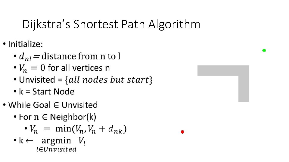
Dijkstra’s Shortest Path Algorithm •

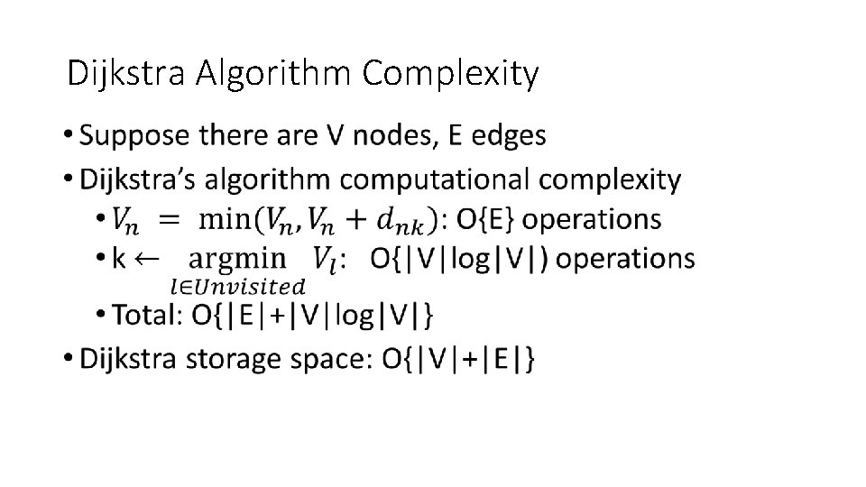
Dijkstra Algorithm Complexity •

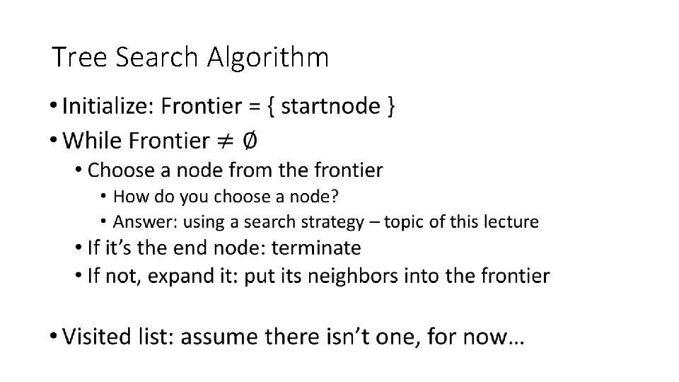
Tree Search Algorithm •

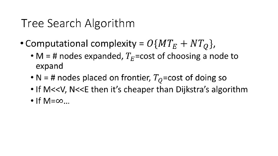
Tree Search Algorithm •

Prioritized Search • Review: Tree Search vs. Dijkstra’s Algorithm • Criteria for evaluating a search algorithm: completeness, optimality, computational cost, storage cost • Search algorithms without side information: BFS, DFS, IDS, UCS • Search algorithms with side information: GBFS vs. A* • • • Heuristics to guide search Greedy best-first search A* search Admissible vs. Consistent heuristics Designing heuristics: Relaxed problem, Sub-problem, Dominance, Max

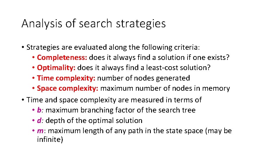
Analysis of search strategies • Strategies are evaluated along the following criteria: • Completeness: does it always find a solution if one exists? • Optimality: does it always find a least-cost solution? • Time complexity: number of nodes generated • Space complexity: maximum number of nodes in memory • Time and space complexity are measured in terms of • b: maximum branching factor of the search tree • d: depth of the optimal solution • m: maximum length of any path in the state space (may be infinite)

Prioritized Search • Review: Tree Search vs. Dijkstra’s Algorithm • Criteria for evaluating a search algorithm: completeness, optimality, computational cost, storage cost • Search algorithms without side information: BFS, DFS, IDS, UCS • Search algorithms with side information: GBFS vs. A* • • • Heuristics to guide search Greedy best-first search A* search Admissible vs. Consistent heuristics Designing heuristics: Relaxed problem, Sub-problem, Dominance, Max

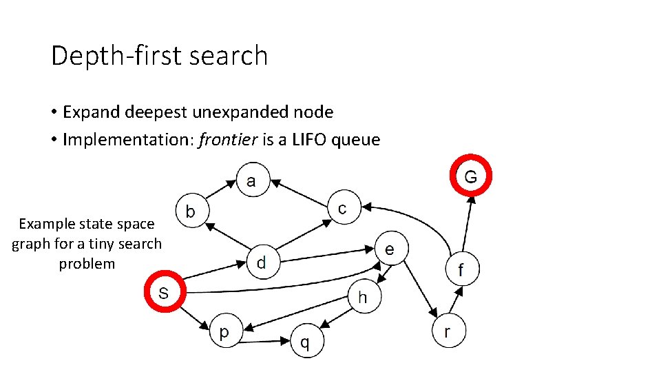
Depth-first search • Expand deepest unexpanded node • Implementation: frontier is a LIFO queue Example state space graph for a tiny search problem

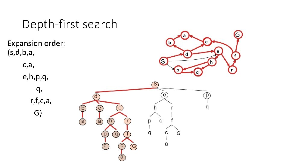
Depth-first search Expansion order: (s, d, b, a, c, a, e, h, p, q, r, f, c, a, G)

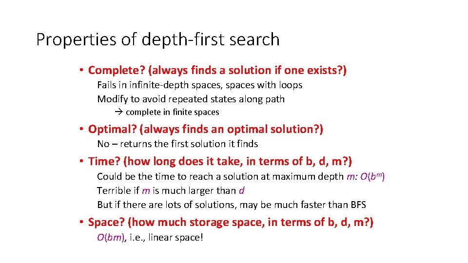
Properties of depth-first search • Complete? (always finds a solution if one exists? ) Fails in infinite-depth spaces, spaces with loops Modify to avoid repeated states along path complete in finite spaces • Optimal? (always finds an optimal solution? ) No – returns the first solution it finds • Time? (how long does it take, in terms of b, d, m? ) Could be the time to reach a solution at maximum depth m: O(bm) Terrible if m is much larger than d But if there are lots of solutions, may be much faster than BFS • Space? (how much storage space, in terms of b, d, m? ) O(bm), i. e. , linear space!

http: //xkcd. com/761/

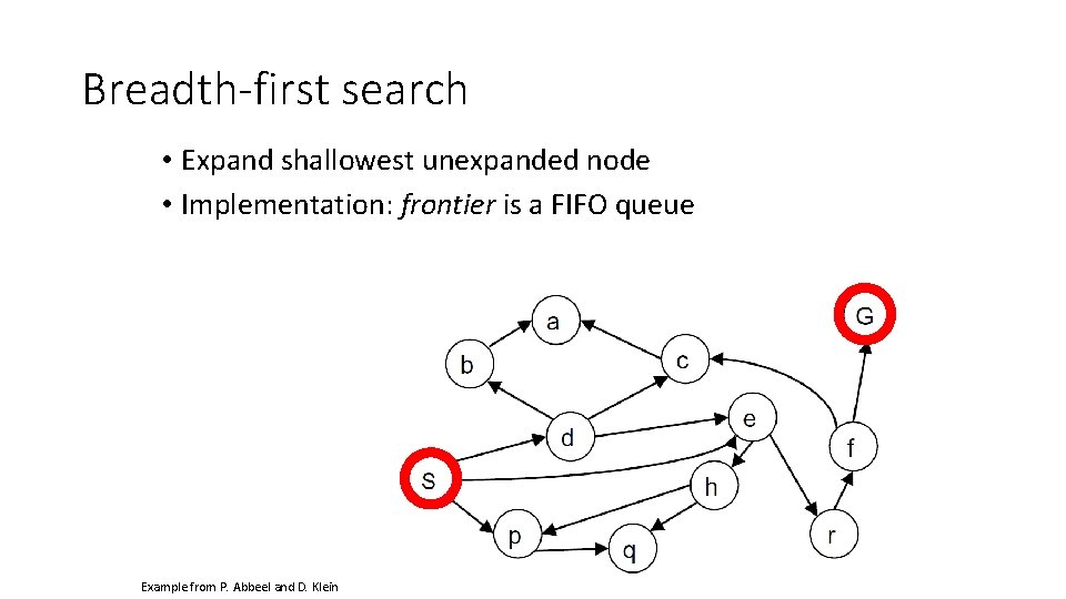
Breadth-first search • Expand shallowest unexpanded node • Implementation: frontier is a FIFO queue Example from P. Abbeel and D. Klein

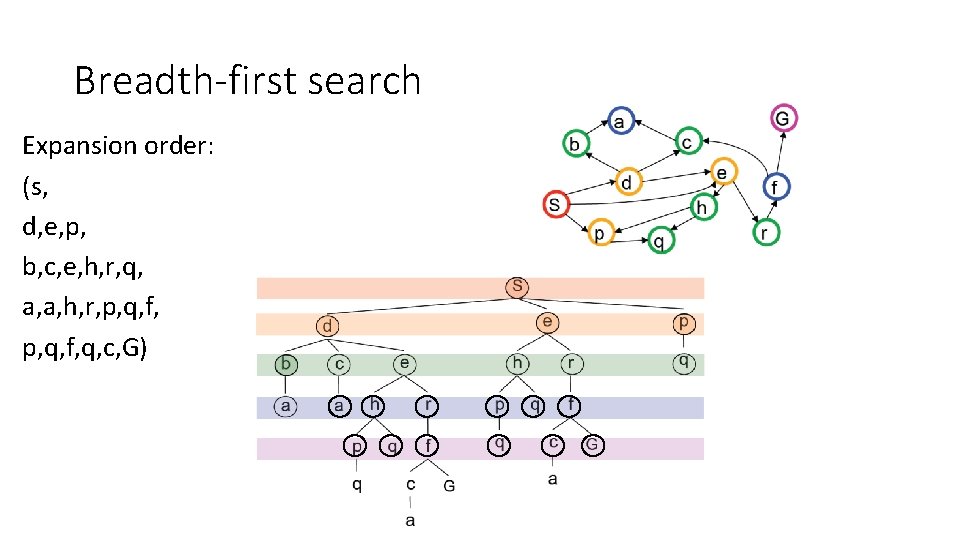
Breadth-first search Expansion order: (s, d, e, p, b, c, e, h, r, q, a, a, h, r, p, q, f, q, c, G)

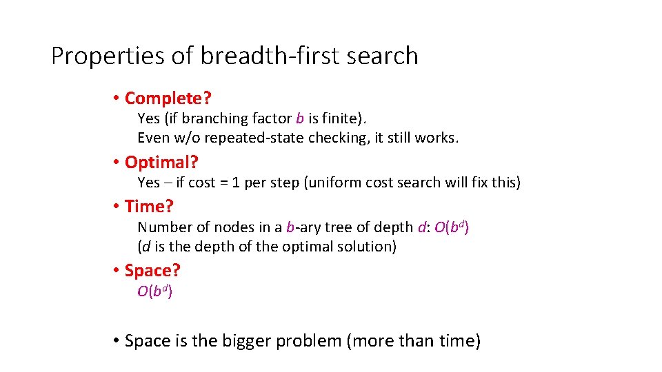
Properties of breadth-first search • Complete? Yes (if branching factor b is finite). Even w/o repeated-state checking, it still works. • Optimal? Yes – if cost = 1 per step (uniform cost search will fix this) • Time? Number of nodes in a b-ary tree of depth d: O(bd) (d is the depth of the optimal solution) • Space? O(bd) • Space is the bigger problem (more than time)

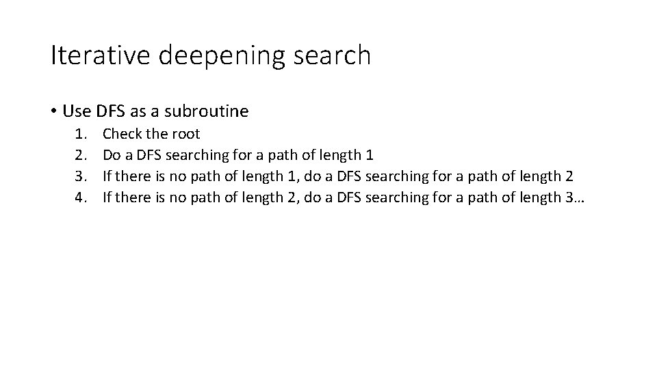
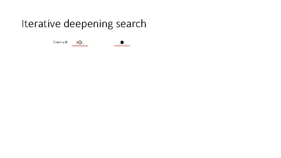
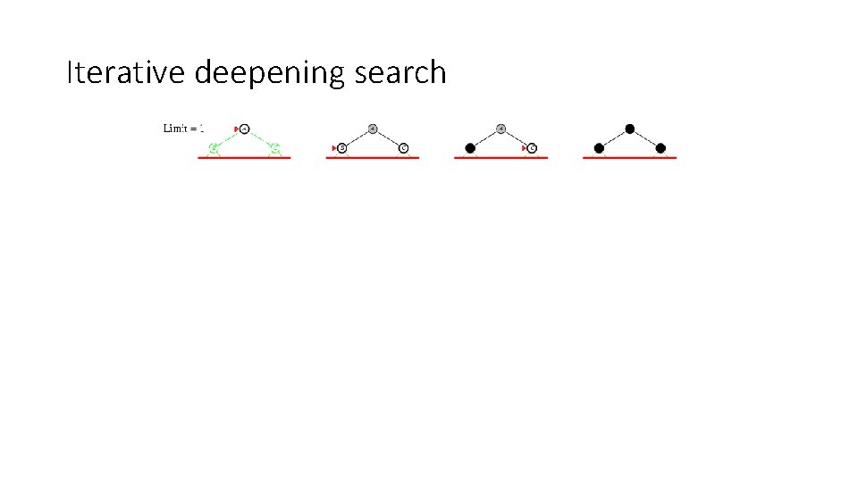
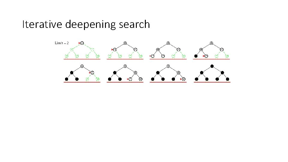
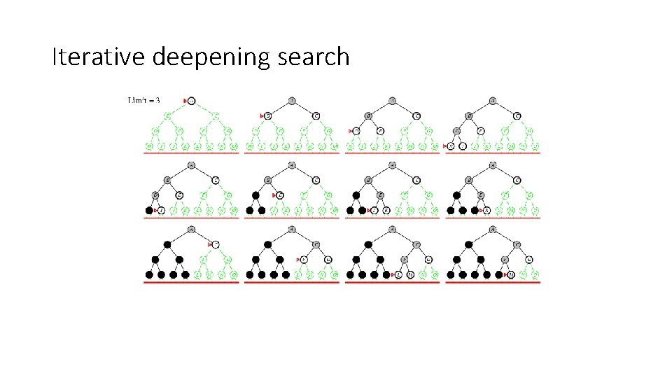
Iterative deepening search • Use DFS as a subroutine 1. 2. 3. 4. Check the root Do a DFS searching for a path of length 1 If there is no path of length 1, do a DFS searching for a path of length 2 If there is no path of length 2, do a DFS searching for a path of length 3…

Iterative deepening search

Iterative deepening search

Iterative deepening search

Iterative deepening search

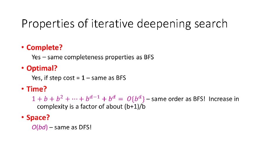
Properties of iterative deepening search •

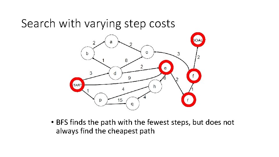
Search with varying step costs • BFS finds the path with the fewest steps, but does not always find the cheapest path

Uniform-cost search • For each frontier node, save the total cost of the path from the initial state to that node • Expand the frontier node with the lowest path cost • Implementation: frontier is a priority queue ordered by path cost • Equivalent to breadth-first if step costs all equal • Equivalent to Dijkstra’s algorithm, if Dijkstra’s algorithm is modified so that a node’s value is computed only when it becomes nonzero

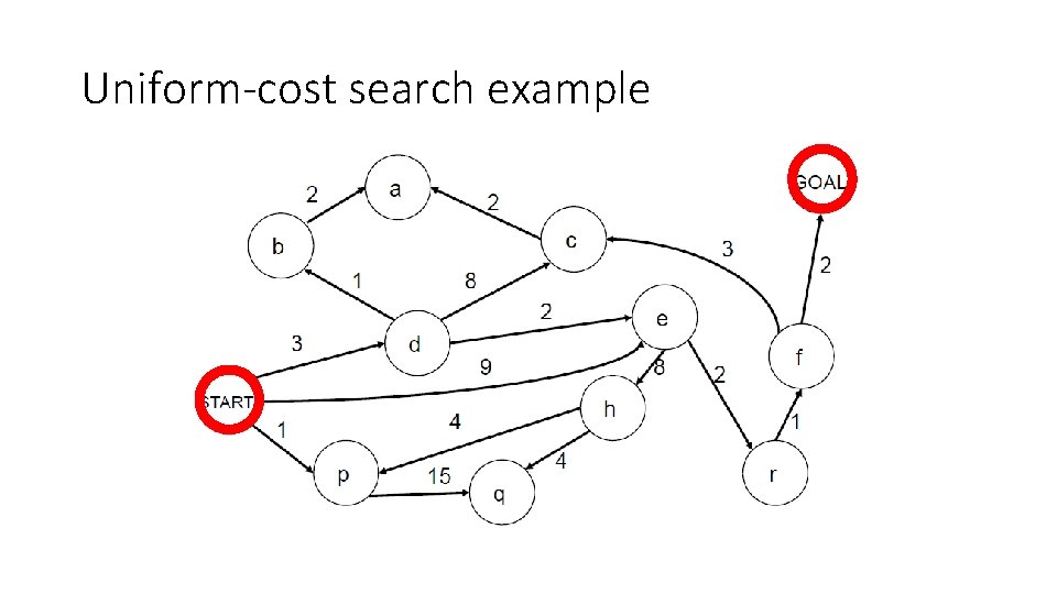
Uniform-cost search example

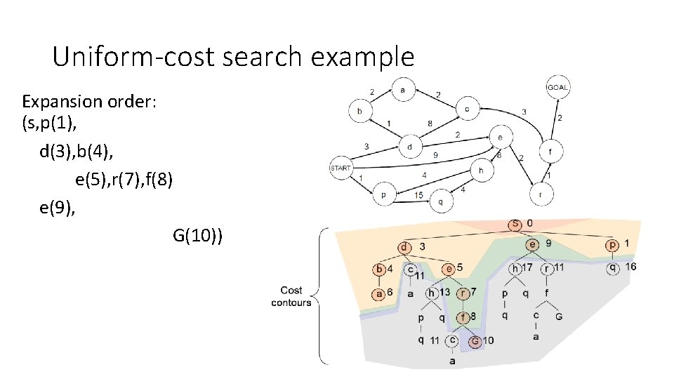
Uniform-cost search example Expansion order: (s, p(1), d(3), b(4), e(5), r(7), f(8) e(9), G(10))

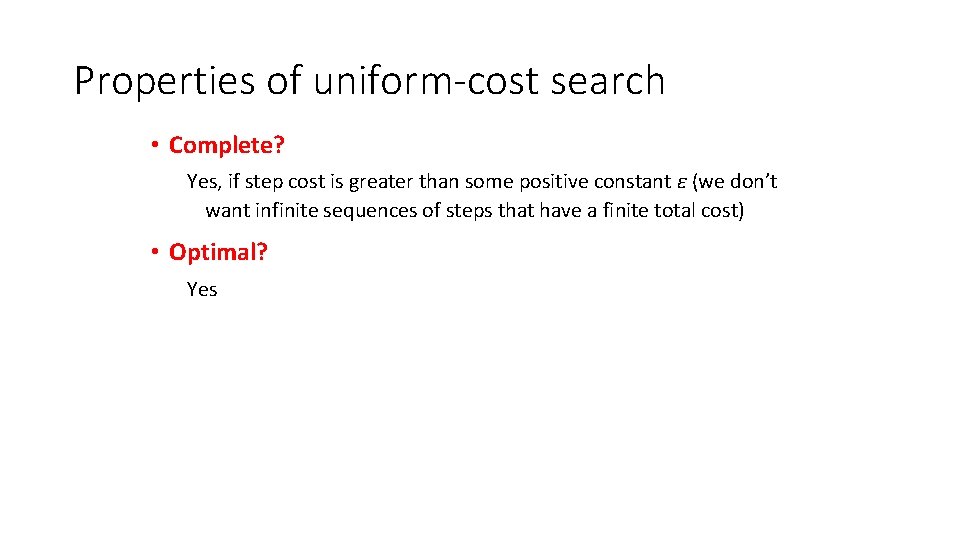
Properties of uniform-cost search • Complete? Yes, if step cost is greater than some positive constant ε (we don’t want infinite sequences of steps that have a finite total cost) • Optimal? Yes

Prioritized Search • Review: Tree Search vs. Dijkstra’s Algorithm • Criteria for evaluating a search algorithm: completeness, optimality, computational cost, storage cost • Search algorithms without side information: BFS, DFS, IDS, UCS • Search algorithms with side information: GBFS vs. A* • • • Heuristics to guide search Greedy best-first search A* search Admissible vs. Consistent heuristics Designing heuristics: Relaxed problem, Sub-problem, Dominance, Max

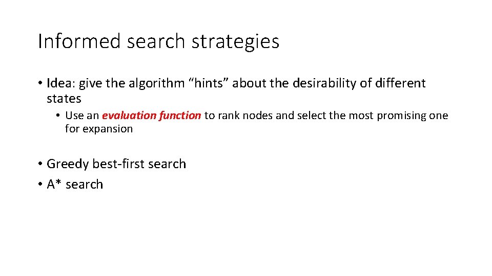
Informed search strategies • Idea: give the algorithm “hints” about the desirability of different states • Use an evaluation function to rank nodes and select the most promising one for expansion • Greedy best-first search • A* search

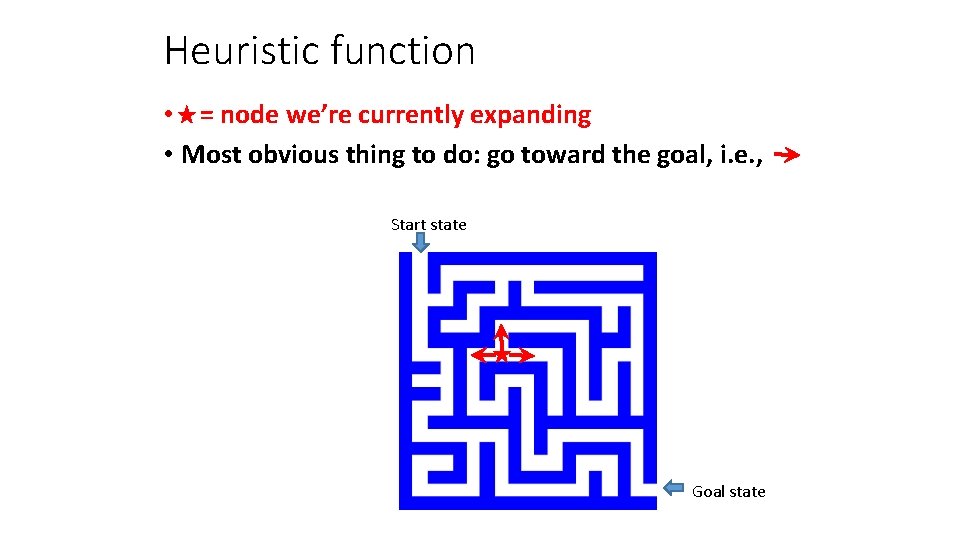
Heuristic function • = node we’re currently expanding • Most obvious thing to do: go toward the goal, i. e. , Start state Goal state

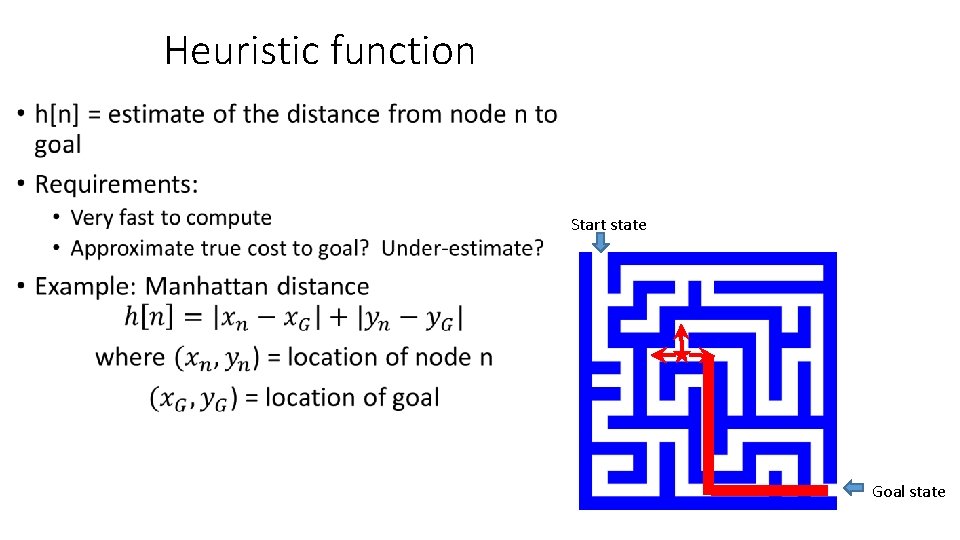
Heuristic function • Start state Goal state

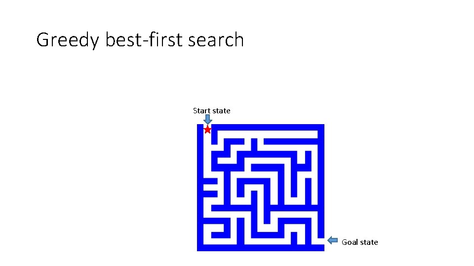
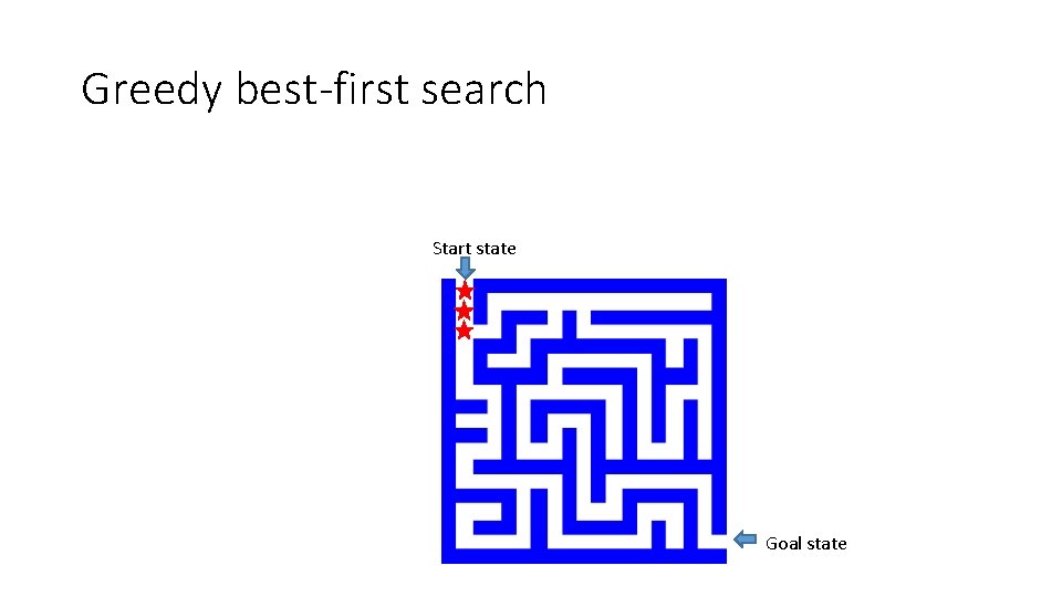
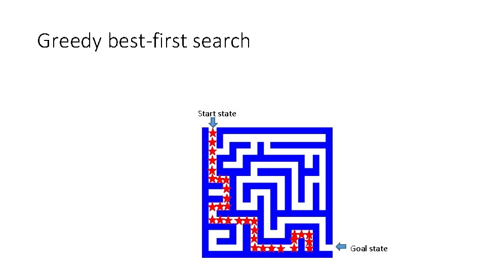
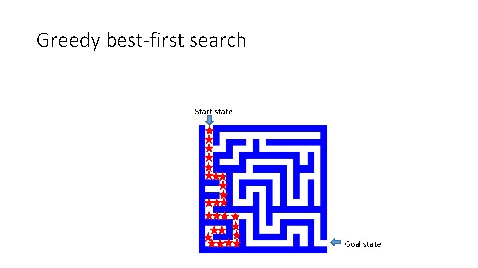
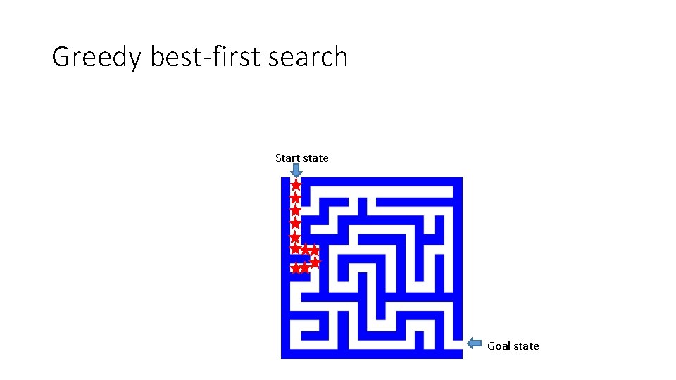
Greedy best-first search Expand the node that has the lowest value of the heuristic function h(n)

Greedy best-first search Start state Goal state

Greedy best-first search Start state Goal state

Greedy best-first search Start state Goal state

Greedy best-first search Start state Goal state

Greedy best-first search Start state Goal state

Greedy best-first search Start state Goal state

Properties of greedy best-first search • Complete? No – can get stuck in loops • Optimal? No • Time? Worst case: O(bm) Can be much better with a good heuristic • Space? Worst case: O(bm)

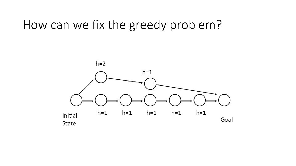
How can we fix the greedy problem?

A* search • Idea: avoid expanding paths that are already expensive • The evaluation function f(n) is the estimated total cost of the path through node n to the goal: f(n) = g(n) + h(n) g(n): cost so far to reach n (path cost) h(n): estimated cost from n to goal (heuristic)

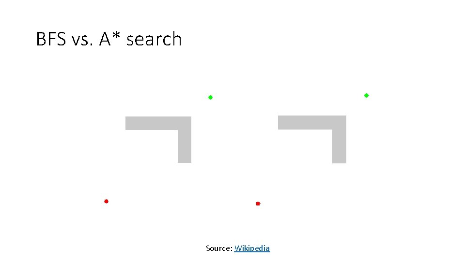
BFS vs. A* search Source: Wikipedia

Admissible heuristics • An admissible heuristic never overestimates the cost to reach the goal • A heuristic h(n) is admissible if for every node n, h(n) ≤ h*(n), where h*(n) is the true cost to reach the goal state from n • Example: • straight line distance never overestimates the actual road distance • Manhattan distance never overestimates actual road distance if all roads are on a Manhattan grid • Theorem: If h(n) is admissible, and if we don’t do repeated-state detection, then A* is optimal

Optimality of A* • Theorem: If h(n) is admissible, A* is optimal (if we don’t do repeated state detection) • Proof sketch: • A* expands all nodes for which f(n) ≤ C*, i. e. , the estimated path cost to the goal is less than or equal to the actual path cost to the first goal encountered • When we reach the goal node, all the other nodes remaining on the frontier have estimated path costs to the goal that are at least as big as C* • Because we are using an admissible heuristic, the true path costs to the goal for these nodes cannot be less than C*

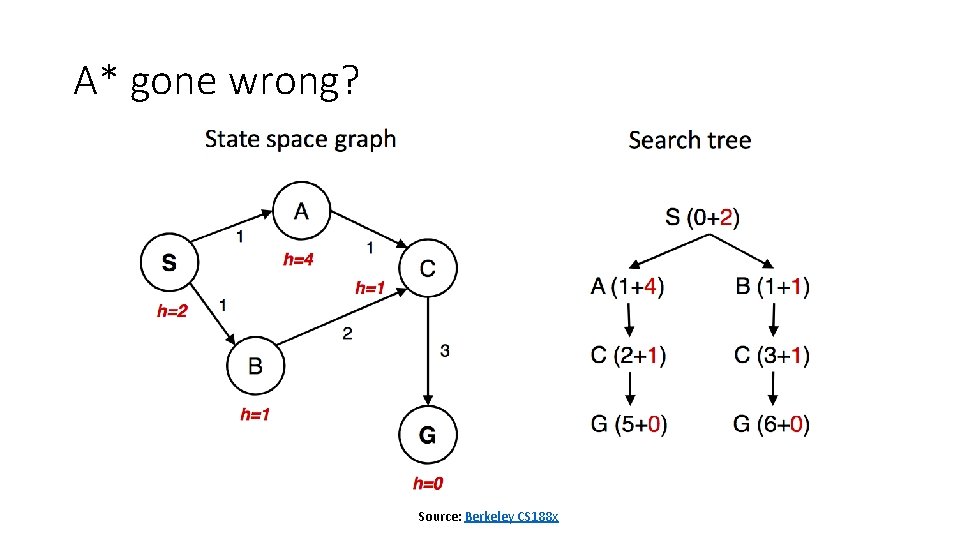
A* gone wrong? Source: Berkeley CS 188 x

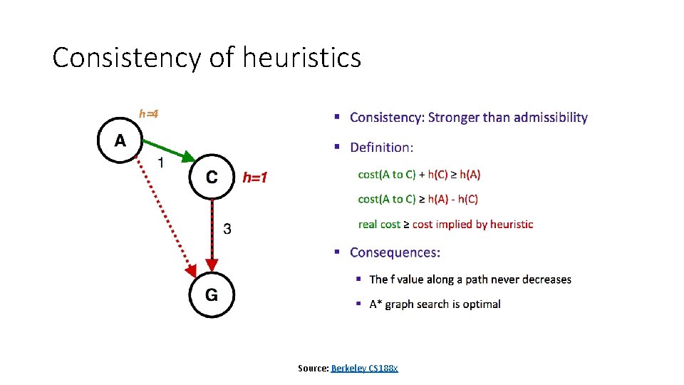
Consistency of heuristics h=4 Source: Berkeley CS 188 x

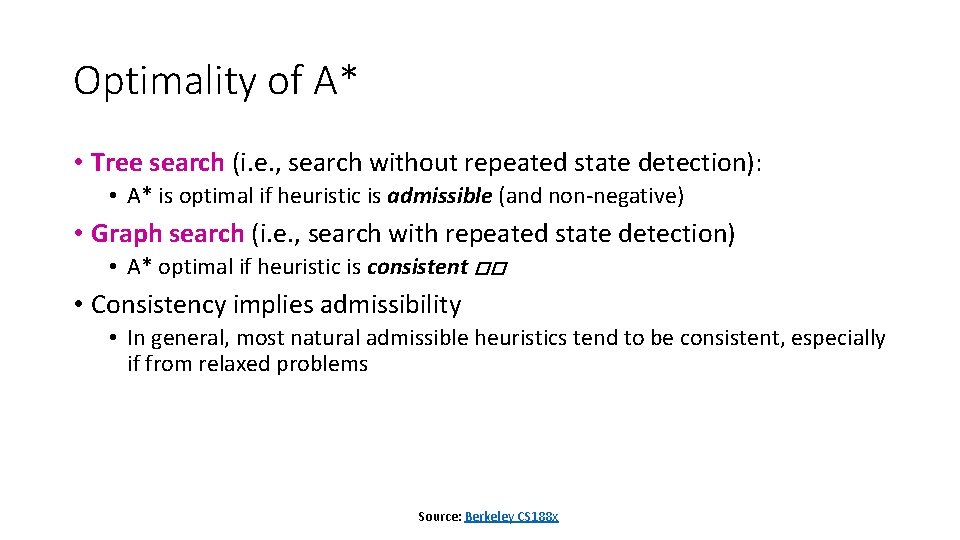
Optimality of A* • Tree search (i. e. , search without repeated state detection): • A* is optimal if heuristic is admissible (and non-negative) • Graph search (i. e. , search with repeated state detection) • A* optimal if heuristic is consistent �� • Consistency implies admissibility • In general, most natural admissible heuristics tend to be consistent, especially if from relaxed problems Source: Berkeley CS 188 x

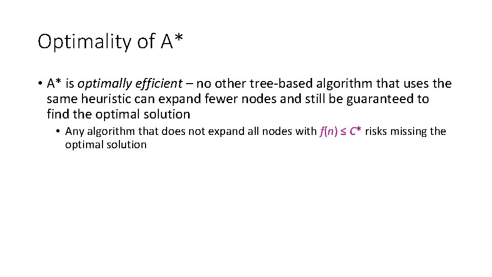
Optimality of A* • A* is optimally efficient – no other tree-based algorithm that uses the same heuristic can expand fewer nodes and still be guaranteed to find the optimal solution • Any algorithm that does not expand all nodes with f(n) ≤ C* risks missing the optimal solution

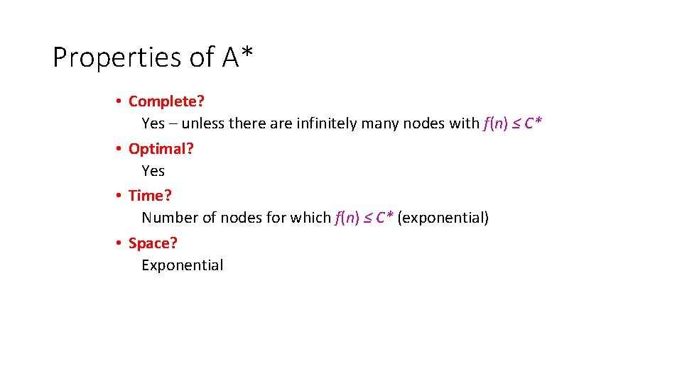
Properties of A* • Complete? Yes – unless there are infinitely many nodes with f(n) ≤ C* • Optimal? Yes • Time? Number of nodes for which f(n) ≤ C* (exponential) • Space? Exponential

Prioritized Search • Review: Tree Search vs. Dijkstra’s Algorithm • Criteria for evaluating a search algorithm: completeness, optimality, computational cost, storage cost • Search algorithms without side information: BFS, DFS, IDS, UCS • Search algorithms with side information: GBFS vs. A* • • • Heuristics to guide search Greedy best-first search A* search Admissible vs. Consistent heuristics Designing heuristics: Relaxed problem, Sub-problem, Dominance, Max

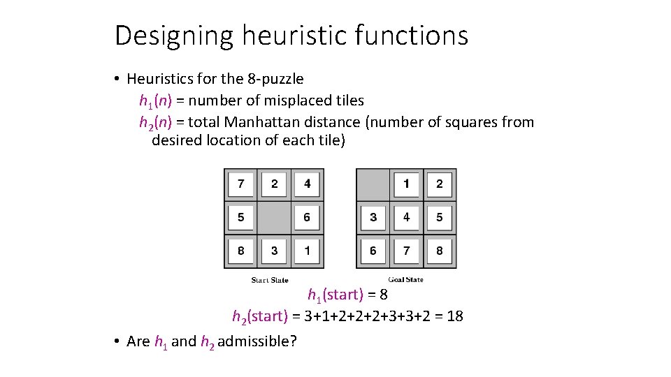
Designing heuristic functions • Heuristics for the 8 -puzzle h 1(n) = number of misplaced tiles h 2(n) = total Manhattan distance (number of squares from desired location of each tile) h 1(start) = 8 h 2(start) = 3+1+2+2+2+3+3+2 = 18 • Are h 1 and h 2 admissible?

Heuristics from relaxed problems • A problem with fewer restrictions on the actions is called a relaxed problem • The cost of an optimal solution to a relaxed problem is an admissible heuristic for the original problem • If the rules of the 8 -puzzle are relaxed so that a tile can move anywhere, then h 1(n) gives the shortest solution • If the rules are relaxed so that a tile can move to any adjacent square, then h 2(n) gives the shortest solution

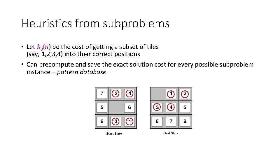
Heuristics from subproblems • Let h 3(n) be the cost of getting a subset of tiles (say, 1, 2, 3, 4) into their correct positions • Can precompute and save the exact solution cost for every possible subproblem instance – pattern database

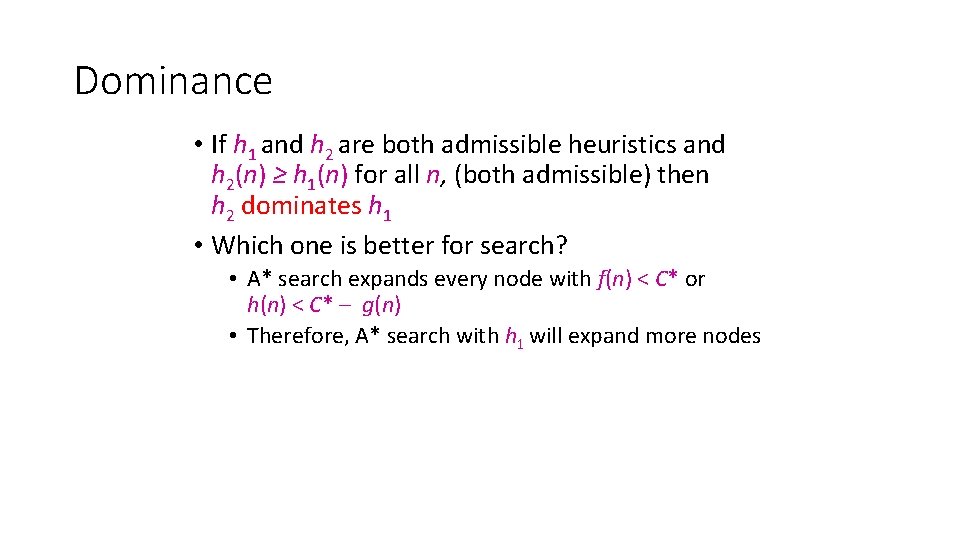
Dominance • If h 1 and h 2 are both admissible heuristics and h 2(n) ≥ h 1(n) for all n, (both admissible) then h 2 dominates h 1 • Which one is better for search? • A* search expands every node with f(n) < C* or h(n) < C* – g(n) • Therefore, A* search with h 1 will expand more nodes

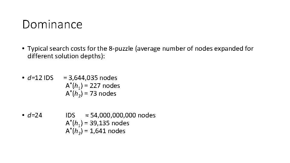
Dominance • Typical search costs for the 8 -puzzle (average number of nodes expanded for different solution depths): • d=12 IDS = 3, 644, 035 nodes A*(h 1) = 227 nodes A*(h 2) = 73 nodes • d=24 IDS ≈ 54, 000, 000 nodes A*(h 1) = 39, 135 nodes A*(h 2) = 1, 641 nodes

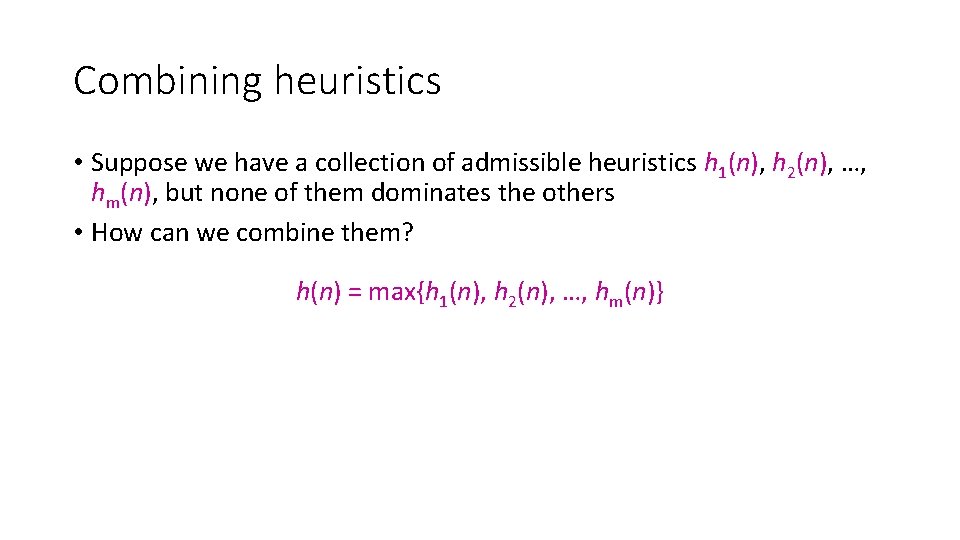
Combining heuristics • Suppose we have a collection of admissible heuristics h 1(n), h 2(n), …, hm(n), but none of them dominates the others • How can we combine them? h(n) = max{h 1(n), h 2(n), …, hm(n)}

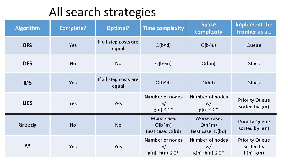
All search strategies Algorithm Complete? Optimal? Time complexity Space complexity Implement the Frontier as a… BFS Yes If all step costs are equal O(b^d) Queue DFS No No O(b^m) O(bm) Stack IDS Yes If all step costs are equal O(b^d) O(bd) Stack Yes Number of nodes w/ g(n) ≤ C* Priority Queue sorted by g(n) No Worst case: O(b^m) Best case: O(bd) Worse case: O(b^m) Best case: O(bd) Priority Queue sorted by h(n) Yes Number of nodes w/ g(n)+h(n) ≤ C* Priority Queue sorted by h(n)+g(n) UCS Greedy A* Yes No Yes