CS 440ECE 448 Lecture 3 Search Order Slides

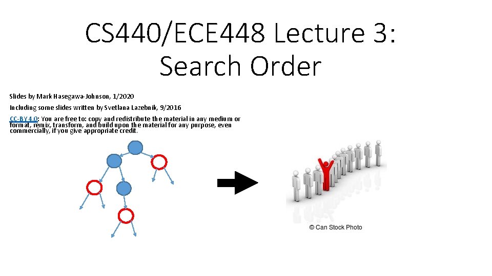
CS 440/ECE 448 Lecture 3: Search Order Slides by Mark Hasegawa-Johnson, 1/2020 Including some slides written by Svetlana Lazebnik, 9/2016 CC-BY 4. 0: You are free to: copy and redistribute the material in any medium or format, remix, transform, and build upon the material for any purpose, even commercially, if you give appropriate credit.

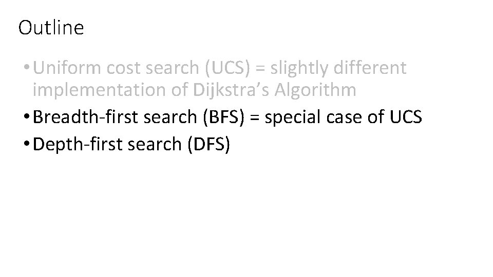
Outline • Uniform cost search (UCS) = slightly different implementation of Dijkstra’s Algorithm • Breadth-first search (BFS) = special case of UCS • Depth-first search (DFS)

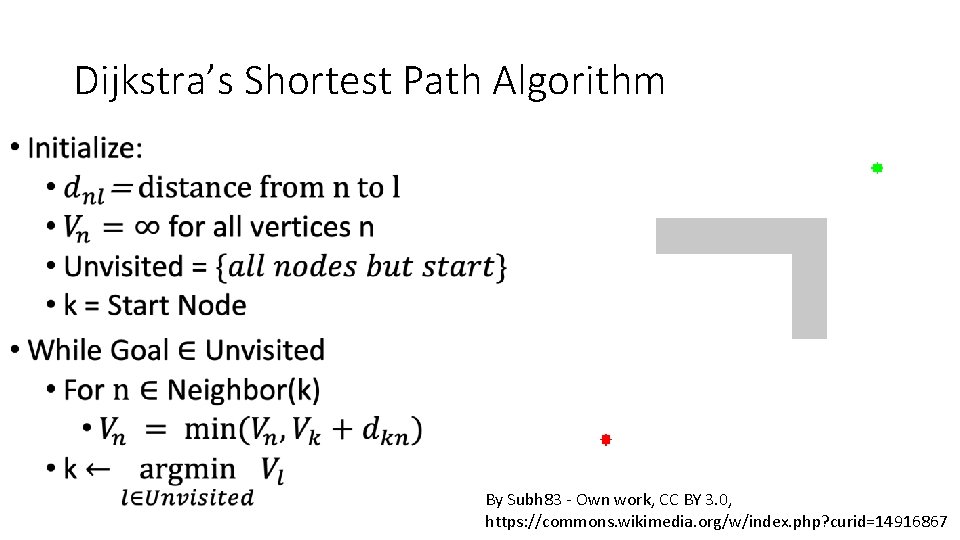
Dijkstra’s Shortest Path Algorithm • By Subh 83 - Own work, CC BY 3. 0, https: //commons. wikimedia. org/w/index. php? curid=14916867

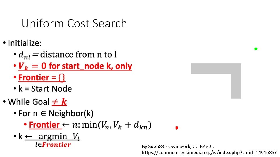
Uniform Cost Search • By Subh 83 - Own work, CC BY 3. 0, https: //commons. wikimedia. org/w/index. php? curid=14916867

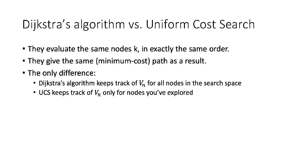
Dijkstra’s algorithm vs. Uniform Cost Search •

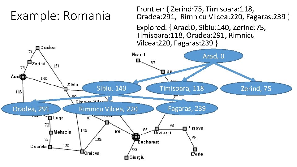
Example: Romania Frontier: { Zerind: 75, Timisoara: 118, Oradea: 291, Rimnicu Vilcea: 220, Fagaras: 239 } Explored: { Arad: 0, Sibiu: 140, Zerind: 75, Timisoara: 118, Oradea: 291, Rimnicu Vilcea: 220, Fagaras: 239 } Arad, 0 Sibiu, 140 Oradea, 291 Rimnicu Vilcea, 220 Timisoara, 118 Fagaras, 239 Zerind, 75

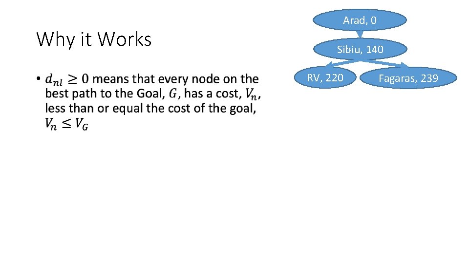
Why it Works • Arad, 0 Sibiu, 140 RV, 220 Fagaras, 239

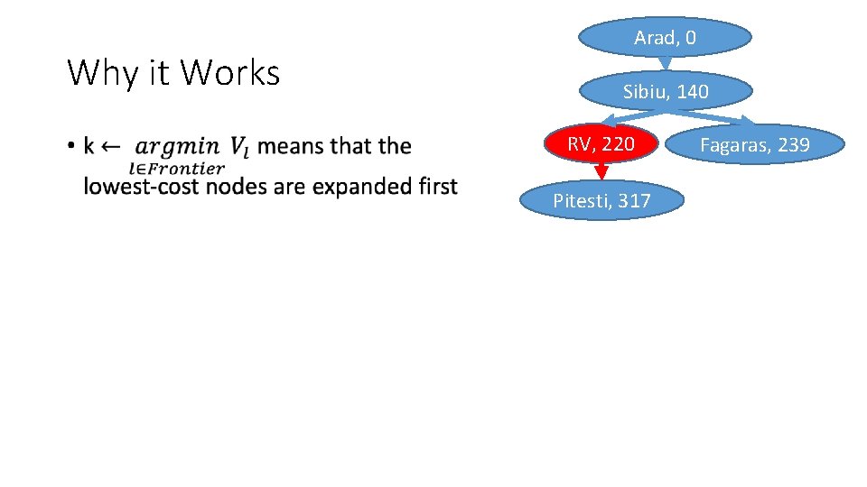
Why it Works • Arad, 0 Sibiu, 140 RV, 220 Pitesti, 317 Fagaras, 239

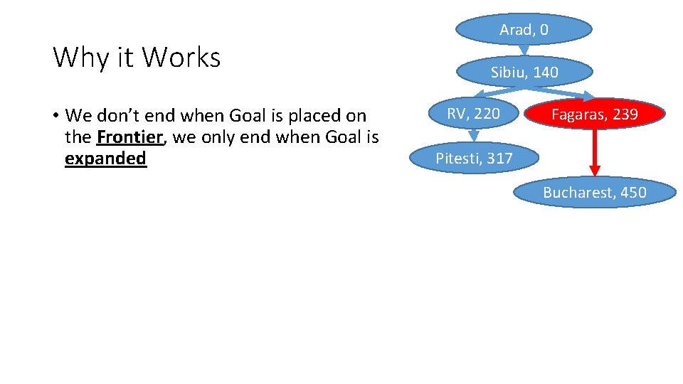
Why it Works • We don’t end when Goal is placed on the Frontier, we only end when Goal is expanded Arad, 0 Sibiu, 140 RV, 220 Fagaras, 239 Pitesti, 317 Bucharest, 450

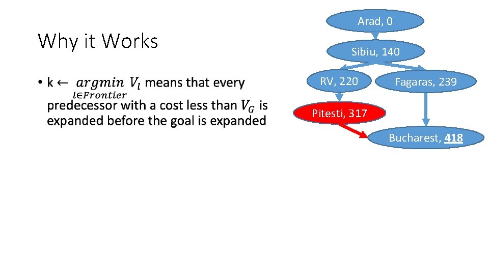
Why it Works • Arad, 0 Sibiu, 140 RV, 220 Fagaras, 239 Pitesti, 317 Bucharest, 418

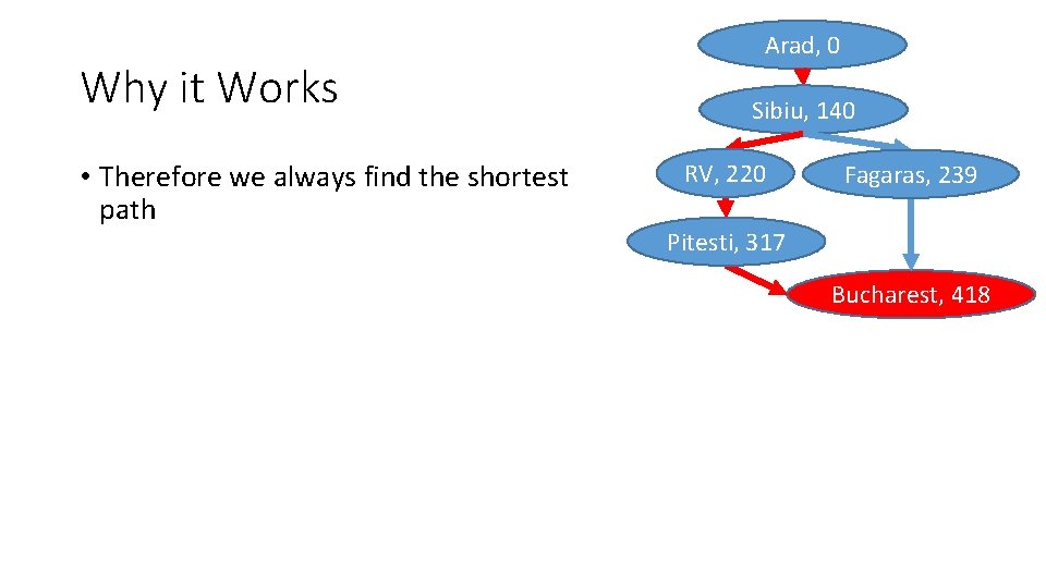
Why it Works • Therefore we always find the shortest path Arad, 0 Sibiu, 140 RV, 220 Fagaras, 239 Pitesti, 317 Bucharest, 418

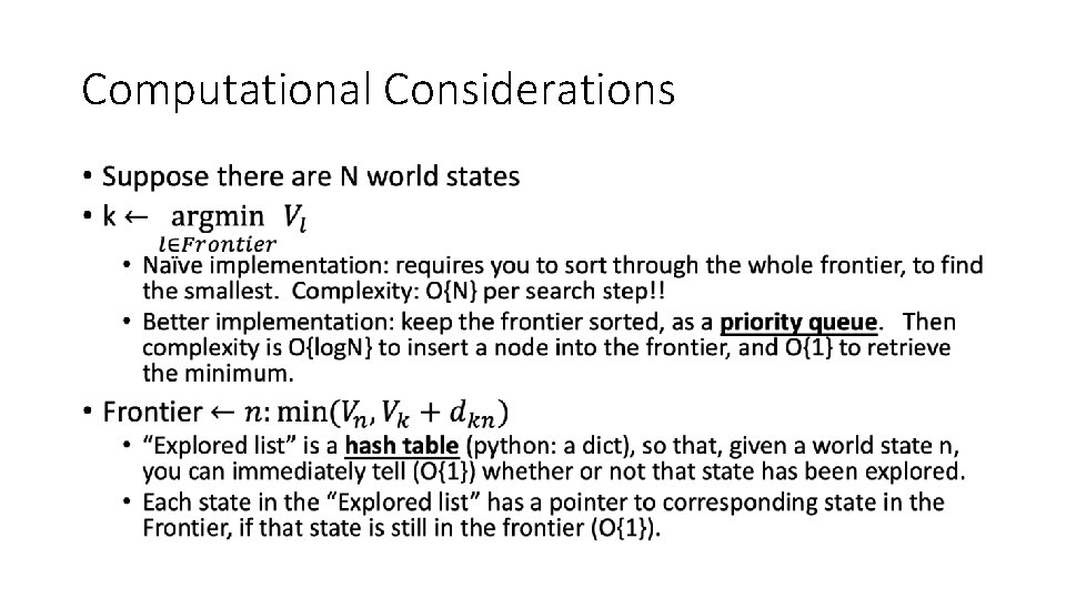
Computational Considerations •

Outline • Uniform cost search (UCS) = slightly different implementation of Dijkstra’s Algorithm • Breadth-first search (BFS) = special case of UCS • Depth-first search (DFS)

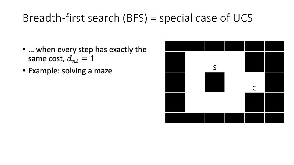
Breadth-first search (BFS) = special case of UCS • S G

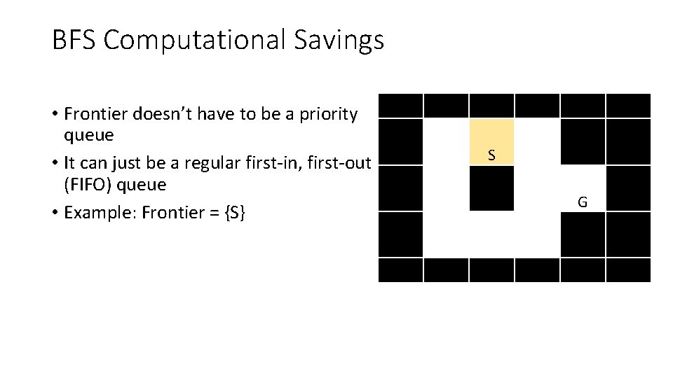
BFS Computational Savings • Frontier doesn’t have to be a priority queue • It can just be a regular first-in, first-out (FIFO) queue • Example: Frontier = {S} S G

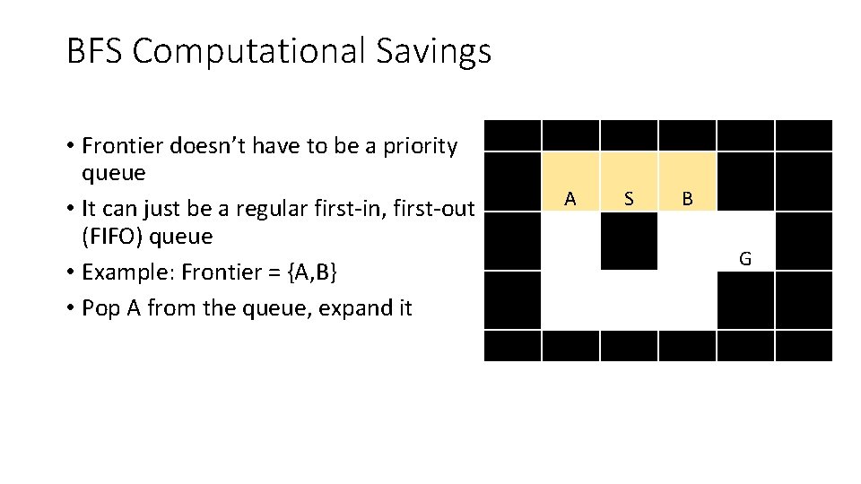
BFS Computational Savings • Frontier doesn’t have to be a priority queue • It can just be a regular first-in, first-out (FIFO) queue • Example: Frontier = {A, B} • Pop A from the queue, expand it A S B G

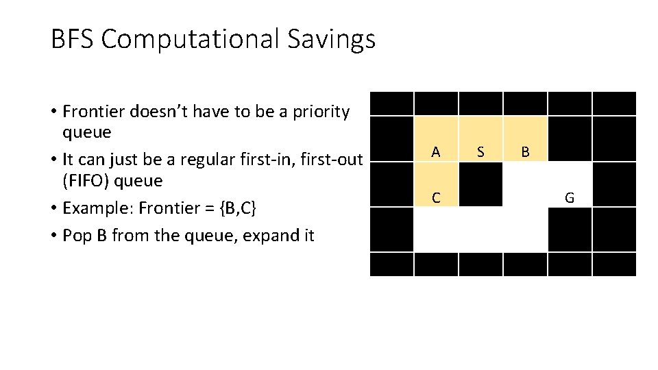
BFS Computational Savings • Frontier doesn’t have to be a priority queue • It can just be a regular first-in, first-out (FIFO) queue • Example: Frontier = {B, C} • Pop B from the queue, expand it A C S B G

BFS Computational Savings • Frontier doesn’t have to be a priority queue • It can just be a regular first-in, first-out (FIFO) queue • Example: Frontier = {C, D} • Pop C from the queue, expand it A C S B D G

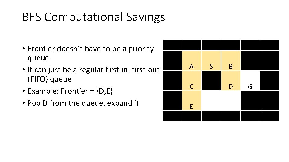
BFS Computational Savings • Frontier doesn’t have to be a priority queue • It can just be a regular first-in, first-out (FIFO) queue • Example: Frontier = {D, E} • Pop D from the queue, expand it A C E S B D G

BFS Computational Savings • Frontier doesn’t have to be a priority queue • It can just be a regular first-in, first-out (FIFO) queue • Example: Frontier = {E, G} • Pop E from the queue, expand it A C E S B D G

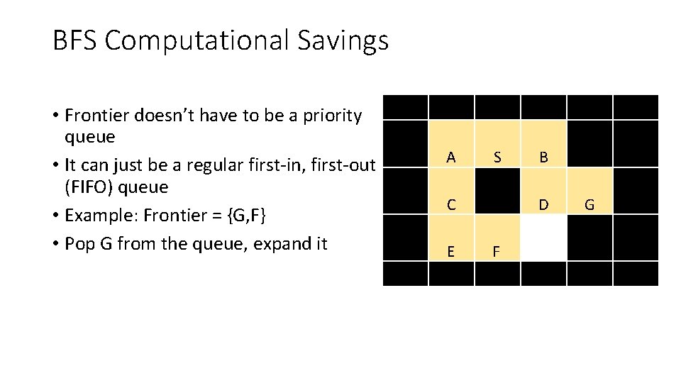
BFS Computational Savings • Frontier doesn’t have to be a priority queue • It can just be a regular first-in, first-out (FIFO) queue • Example: Frontier = {G, F} • Pop G from the queue, expand it A S C E B D F G

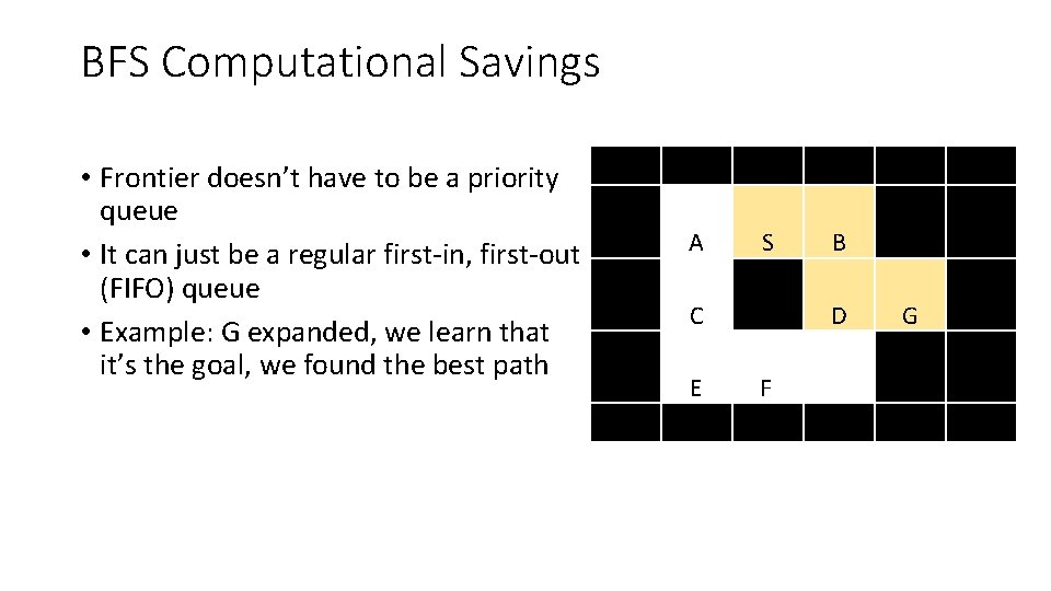
BFS Computational Savings • Frontier doesn’t have to be a priority queue • It can just be a regular first-in, first-out (FIFO) queue • Example: G expanded, we learn that it’s the goal, we found the best path A S C E B D F G

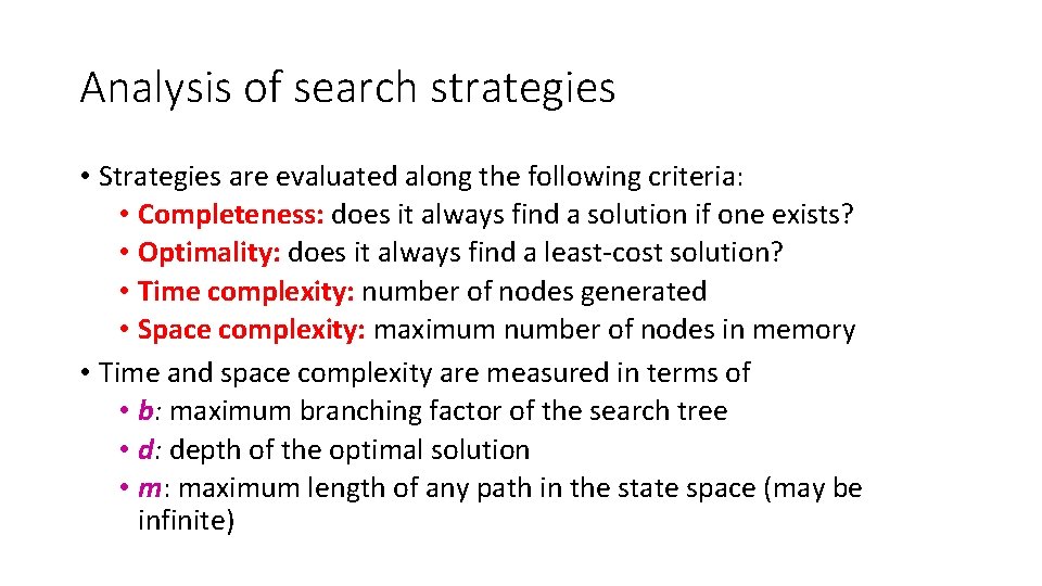
Analysis of search strategies • Strategies are evaluated along the following criteria: • Completeness: does it always find a solution if one exists? • Optimality: does it always find a least-cost solution? • Time complexity: number of nodes generated • Space complexity: maximum number of nodes in memory • Time and space complexity are measured in terms of • b: maximum branching factor of the search tree • d: depth of the optimal solution • m: maximum length of any path in the state space (may be infinite)

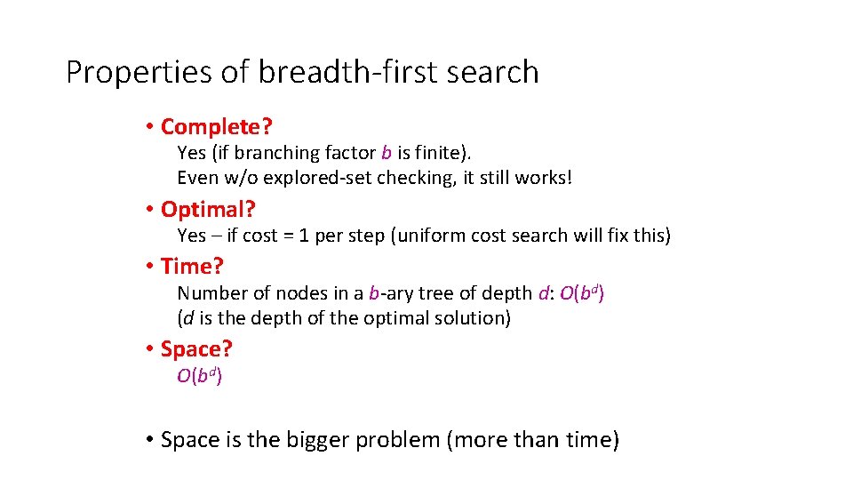
Properties of breadth-first search • Complete? Yes (if branching factor b is finite). Even w/o explored-set checking, it still works! • Optimal? Yes – if cost = 1 per step (uniform cost search will fix this) • Time? Number of nodes in a b-ary tree of depth d: O(bd) (d is the depth of the optimal solution) • Space? O(bd) • Space is the bigger problem (more than time)

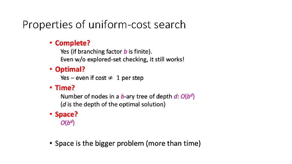
Properties of uniform-cost search •

Outline • Uniform cost search (UCS) = slightly different implementation of Dijkstra’s Algorithm • Breadth-first search (BFS) = special case of UCS • Depth-first search (DFS)

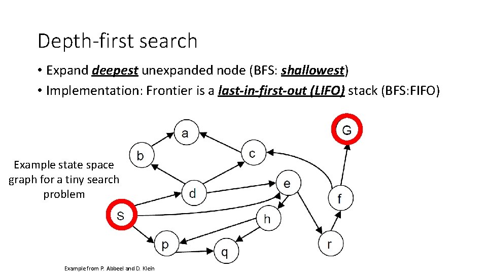
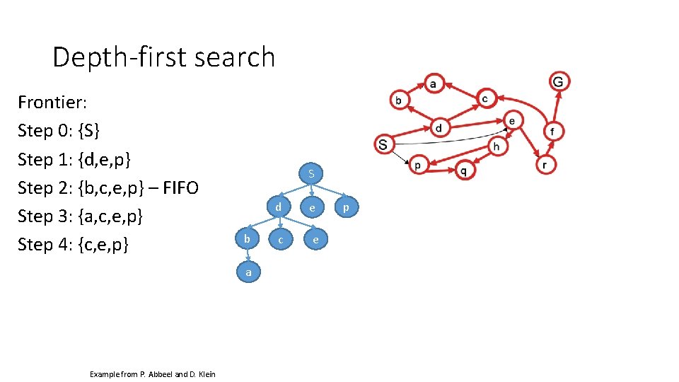
Depth-first search • Expand deepest unexpanded node (BFS: shallowest) • Implementation: Frontier is a last-in-first-out (LIFO) stack (BFS: FIFO) Example state space graph for a tiny search problem Example from P. Abbeel and D. Klein

Depth-first search Frontier: Step 0: {S} Step 1: {d, e, p} Step 2: {b, c, e, p} – FIFO Step 3: {a, c, e, p} Step 4: {c, e, p} S b a Example from P. Abbeel and D. Klein d e c e p

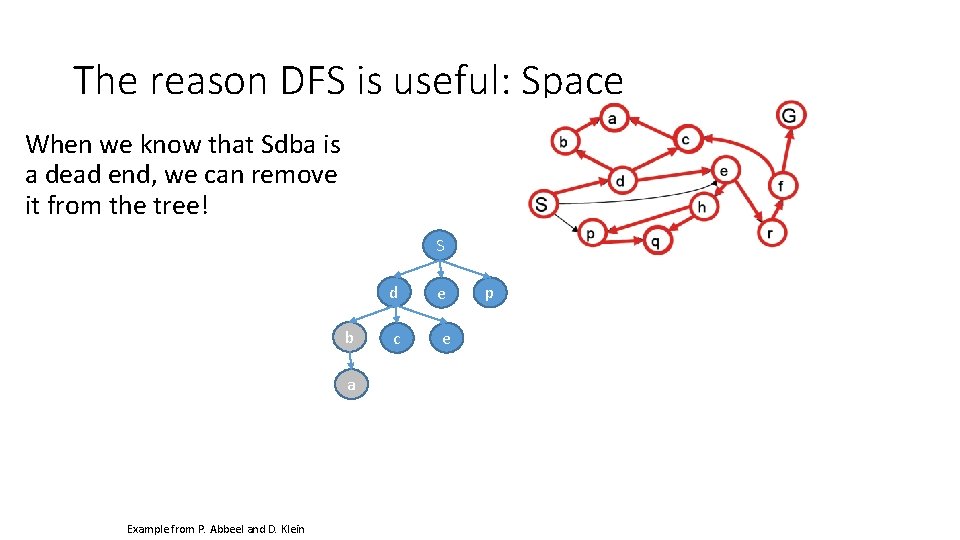
The reason DFS is useful: Space When we know that Sdba is a dead end, we can remove it from the tree! S b a Example from P. Abbeel and D. Klein d e c e p

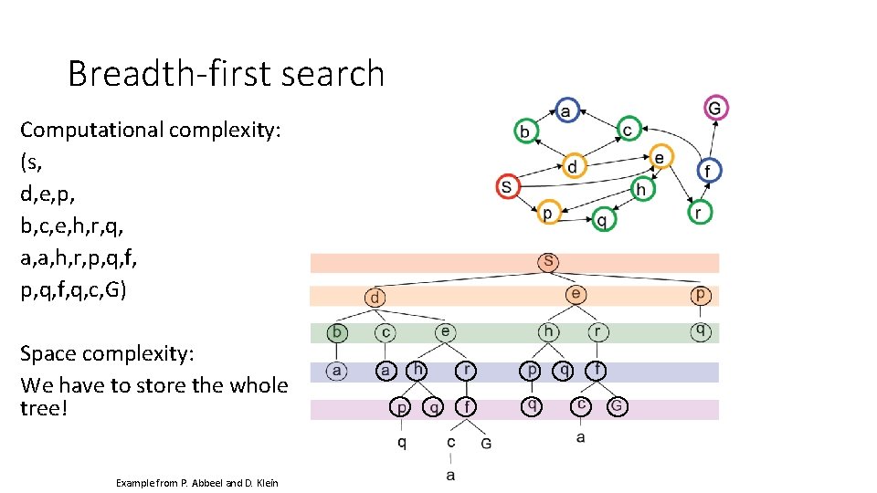
Breadth-first search Computational complexity: (s, d, e, p, b, c, e, h, r, q, a, a, h, r, p, q, f, q, c, G) Space complexity: We have to store the whole tree! Example from P. Abbeel and D. Klein

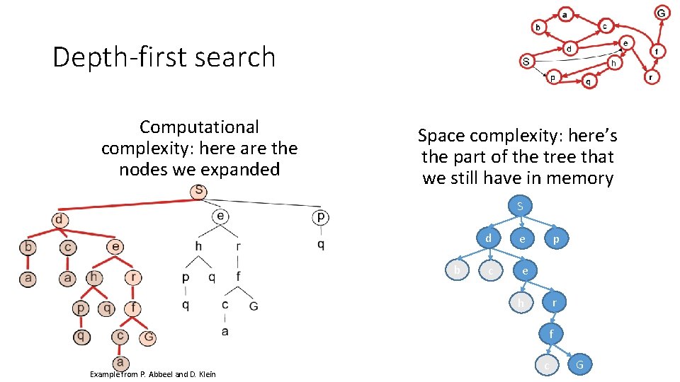
Depth-first search Computational complexity: here are the nodes we expanded Space complexity: here’s the part of the tree that we still have in memory S b d e c e p r h f Example from P. Abbeel and D. Klein c G

Analysis of search strategies • Strategies are evaluated along the following criteria: • Completeness: does it always find a solution if one exists? • Optimality: does it always find a least-cost solution? • Time complexity: number of nodes generated • Space complexity: maximum number of nodes in memory • Time and space complexity are measured in terms of • b: maximum branching factor of the search tree • d: depth of the optimal solution • m: maximum length of any path in the state space (may be infinite)

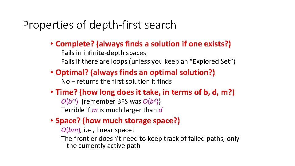
Properties of depth-first search • Complete? (always finds a solution if one exists? ) Fails in infinite-depth spaces Fails if there are loops (unless you keep an “Explored Set”) • Optimal? (always finds an optimal solution? ) No – returns the first solution it finds • Time? (how long does it take, in terms of b, d, m? ) O(bm) (remember BFS was O(bd)) Terrible if m is much larger than d • Space? (how much storage space? ) O(bm), i. e. , linear space! The frontier doesn’t need to keep track of failed paths, only the currently active path

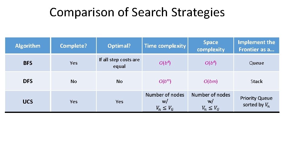
Comparison of Search Strategies Algorithm Complete? Optimal? Time complexity Space complexity Implement the Frontier as a… BFS Yes If all step costs are equal O(bd) Queue DFS No No O(bm) Stack UCS Yes