CPC NOAA Satellite Rainfall Estimation and Applications for

CPC / NOAA: Satellite Rainfall Estimation and Applications for FEWS-NET Nick Novella CPC / NCEP /NOAA Nicholas. Novella@noaa. gov NOAA / FEWS / Chemonics Training Session

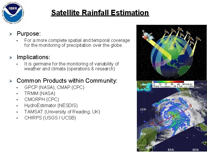
Satellite Rainfall Estimation Ø Purpose: • Ø Implications: • Ø For a more complete spatial and temporal coverage for the monitoring of precipitation over the globe. It is germane for the monitoring of variability of weather and climate (operations & research) Common Products within Community: • • • GPCP (NASA), CMAP (CPC) TRMM (NASA) CMORPH (CPC) Hydro. Estimator (NESDIS) TAMSAT (University of Reading, UK) CHIRPS (USGS / UCSB)

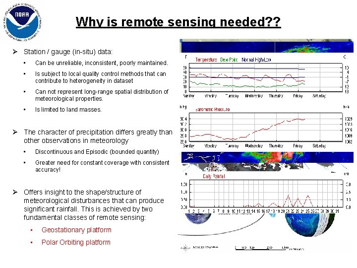
Why is remote sensing needed? ? Ø Station / gauge (in-situ) data: • Can be unreliable, inconsistent, poorly maintained. • Is subject to local quality control methods that can contribute to heterogeneity in dataset • Can not represent long-range spatial distribution of meteorological properties. • Is limited to land masses. Ø The character of precipitation differs greatly than other observations in meteorology • Discontinuous and Episodic (bounded quantity) • Greater need for constant coverage with consistent accuracy! Ø Offers insight to the shape/structure of meteorological disturbances that can produce significant rainfall. This is achieved by two fundamental classes of remote sensing: • Geostationary platform • Polar Orbiting platform

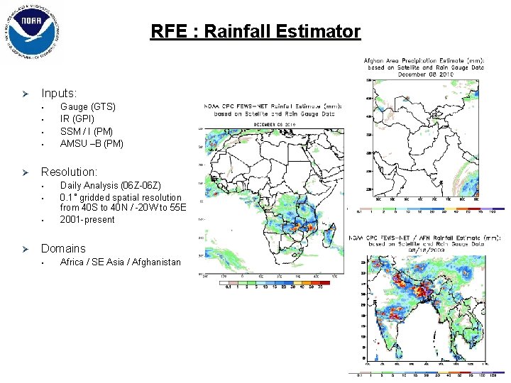
RFE : Rainfall Estimator Ø Inputs: • • Ø Resolution: • • • Ø Gauge (GTS) IR (GPI) SSM / I (PM) AMSU –B (PM) Daily Analysis (06 Z-06 Z) 0. 1˚ gridded spatial resolution from 40 S to 40 N / -20 W to 55 E 2001 -present Domains • Africa / SE Asia / Afghanistan

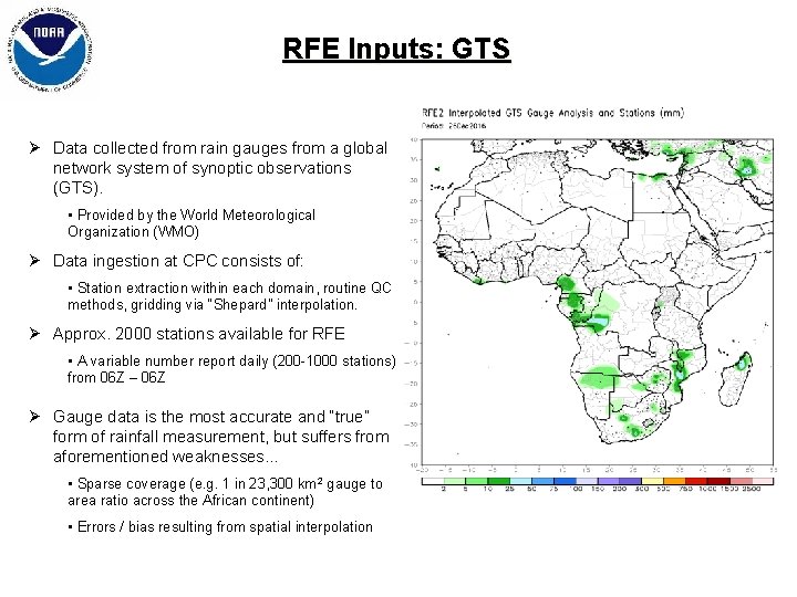
RFE Inputs: GTS Ø Data collected from rain gauges from a global network system of synoptic observations (GTS). • Provided by the World Meteorological Organization (WMO) Ø Data ingestion at CPC consists of: • Station extraction within each domain, routine QC methods, gridding via “Shepard” interpolation. Ø Approx. 2000 stations available for RFE • A variable number report daily (200 -1000 stations) from 06 Z – 06 Z Ø Gauge data is the most accurate and “true” form of rainfall measurement, but suffers from aforementioned weaknesses. . . • Sparse coverage (e. g. 1 in 23, 300 km 2 gauge to area ratio across the African continent) • Errors / bias resulting from spatial interpolation

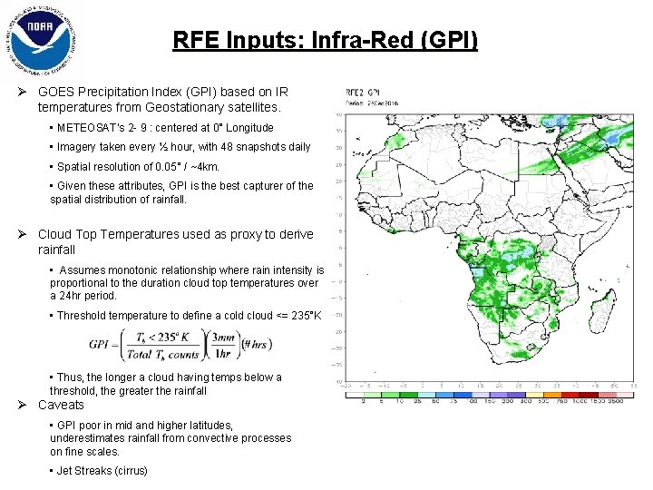
RFE Inputs: Infra-Red (GPI) Ø GOES Precipitation Index (GPI) based on IR temperatures from Geostationary satellites. • METEOSAT’s 2 - 9 : centered at 0° Longitude • Imagery taken every ½ hour, with 48 snapshots daily • Spatial resolution of 0. 05° / ~4 km. • Given these attributes, GPI is the best capturer of the spatial distribution of rainfall. Ø Cloud Top Temperatures used as proxy to derive rainfall • Assumes monotonic relationship where rain intensity is proportional to the duration cloud top temperatures over a 24 hr period. • Threshold temperature to define a cold cloud <= 235°K • Thus, the longer a cloud having temps below a threshold, the greater the rainfall Ø Caveats • GPI poor in mid and higher latitudes, underestimates rainfall from convective processes on fine scales. • Jet Streaks (cirrus)

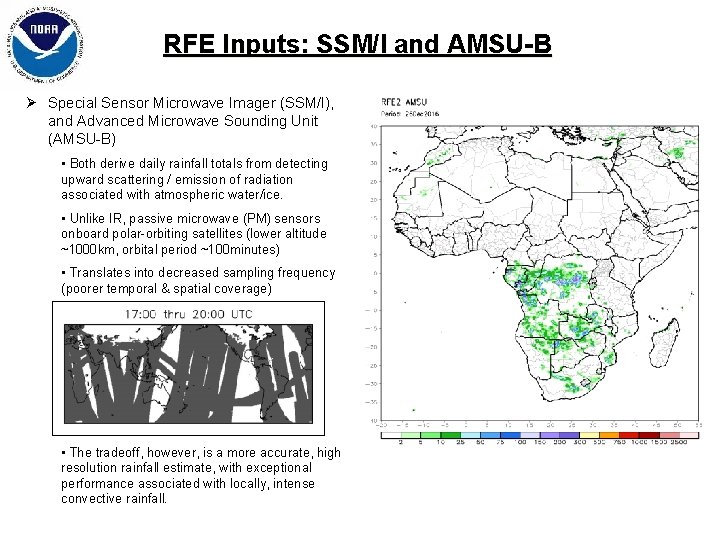
RFE Inputs: SSM/I and AMSU-B Ø Special Sensor Microwave Imager (SSM/I), and Advanced Microwave Sounding Unit (AMSU-B) • Both derive daily rainfall totals from detecting upward scattering / emission of radiation associated with atmospheric water/ice. • Unlike IR, passive microwave (PM) sensors onboard polar-orbiting satellites (lower altitude ~1000 km, orbital period ~100 minutes) • Translates into decreased sampling frequency (poorer temporal & spatial coverage) • The tradeoff, however, is a more accurate, high resolution rainfall estimate, with exceptional performance associated with locally, intense convective rainfall.

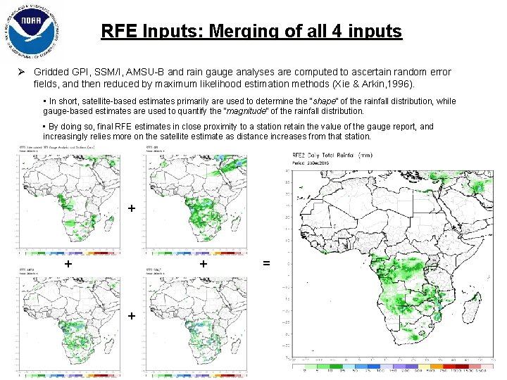
RFE Inputs: Merging of all 4 inputs Ø Gridded GPI, SSM/I, AMSU-B and rain gauge analyses are computed to ascertain random error fields, and then reduced by maximum likelihood estimation methods (Xie & Arkin, 1996). • In short, satellite-based estimates primarily are used to determine the “shape” of the rainfall distribution, while gauge-based estimates are used to quantify the “magnitude” of the rainfall distribution. • By doing so, final RFE estimates in close proximity to a station retain the value of the gauge report, and increasingly relies more on the satellite estimate as distance increases from that station. + + =

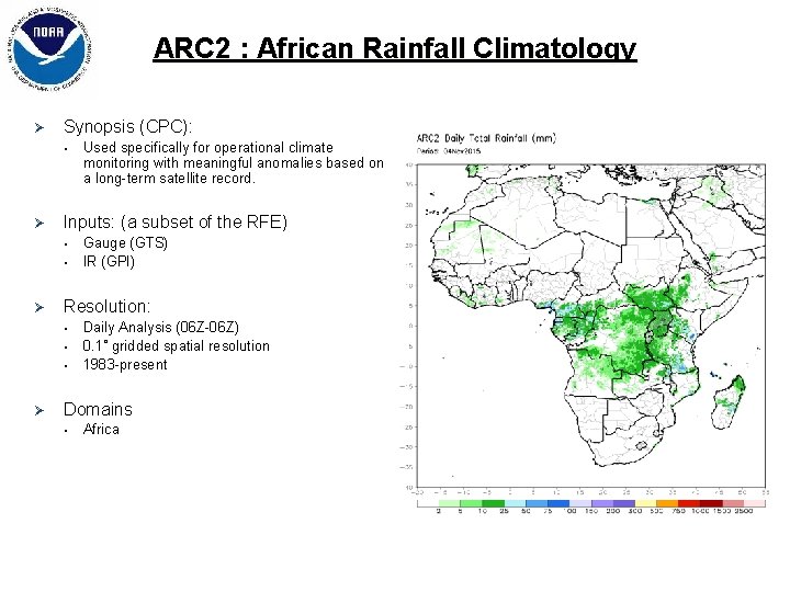
ARC 2 : African Rainfall Climatology Ø Synopsis (CPC): • Ø Inputs: (a subset of the RFE) • • Ø Gauge (GTS) IR (GPI) Resolution: • • • Ø Used specifically for operational climate monitoring with meaningful anomalies based on a long-term satellite record. Daily Analysis (06 Z-06 Z) 0. 1˚ gridded spatial resolution 1983 -present Domains • Africa

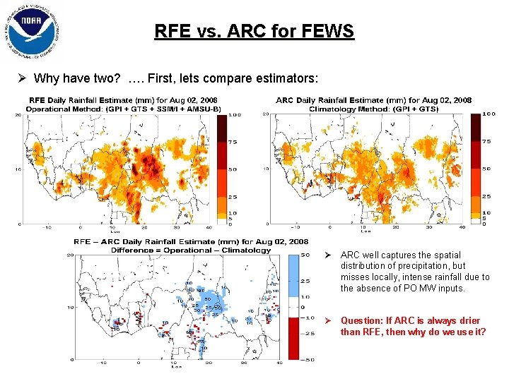
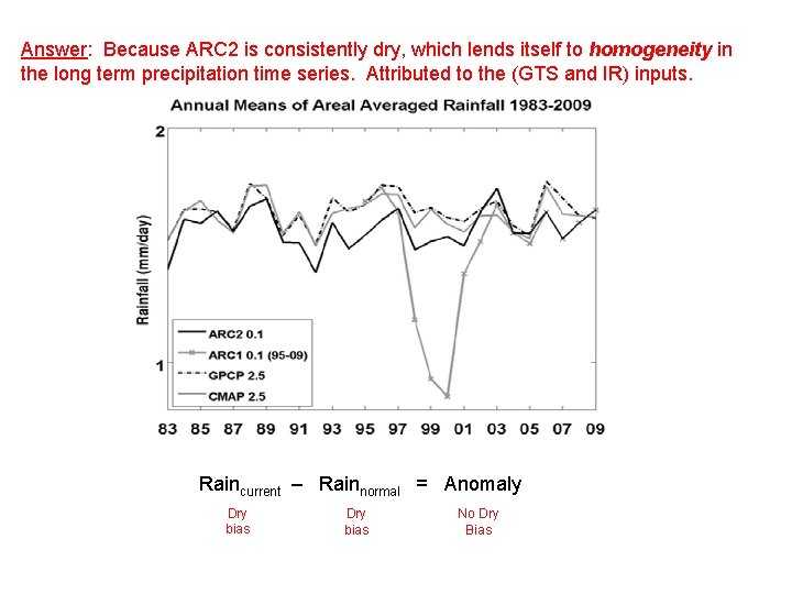
RFE vs. ARC for FEWS Ø Why have two? …. First, lets compare estimators: Ø ARC well captures the spatial distribution of precipitation, but misses locally, intense rainfall due to the absence of PO MW inputs. Ø Question: If ARC is always drier than RFE, then why do we use it?

Answer: Because ARC 2 is consistently dry, which lends itself to homogeneity in the long term precipitation time series. Attributed to the (GTS and IR) inputs. Raincurrent – Rainnormal = Anomaly Dry bias No Dry Bias

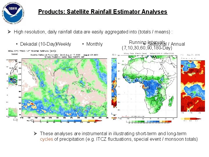
Products: Satellite Rainfall Estimator Analyses Ø High resolution, daily rainfall data are easily aggregated into (totals / means) : • Dekadal (10 -Day)Weekly • Monthly Running Intervals / Annual • Seasonal (7, 10, 30, 60, 90, 180 -Day) Ø These analyses are instrumental in illustrating short-term and long-term cycles of precipitation (e. g. ITCZ fluctuations, special event / monsoon totals)

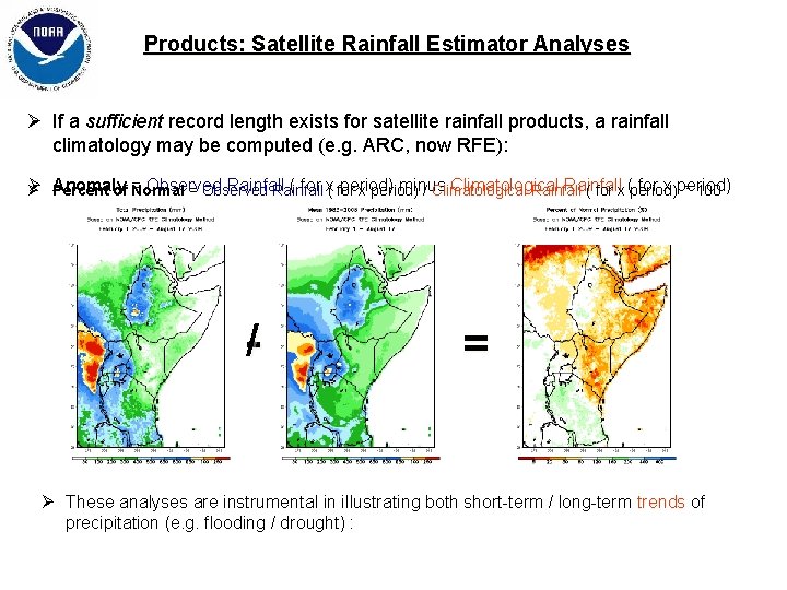
Products: Satellite Rainfall Estimator Analyses Ø If a sufficient record length exists for satellite rainfall products, a rainfall climatology may be computed (e. g. ARC, now RFE): Ø Observed Rainfall ( for x( for period) minus Climatological Rainfall for x period) Ø Anomaly Percent of = Normal = Observed Rainfall x period) / Climatological Rainfall ( for x (period) * 100 -/ = Ø These analyses are instrumental in illustrating both short-term / long-term trends of precipitation (e. g. flooding / drought) :

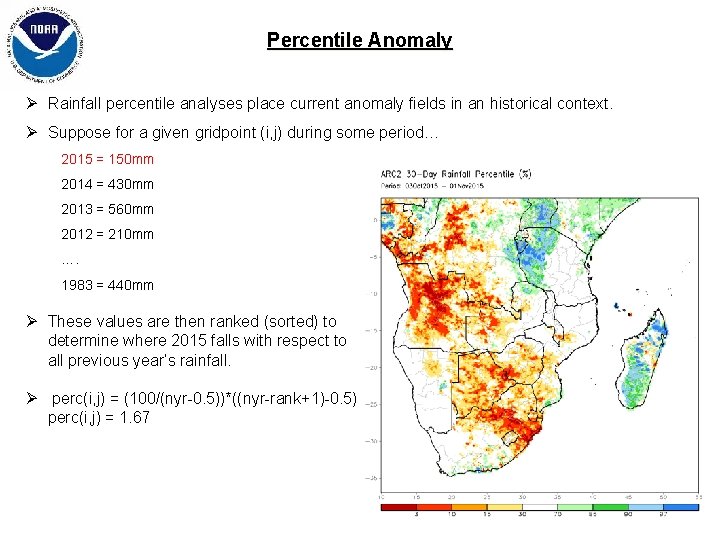
Percentile Anomaly Ø Rainfall percentile analyses place current anomaly fields in an historical context. Ø Suppose for a given gridpoint (i, j) during some period… 2015 = 150 mm 2014 = 430 mm 2013 = 560 mm 2012 = 210 mm …. 1983 = 440 mm Ø These values are then ranked (sorted) to determine where 2015 falls with respect to all previous year’s rainfall. Ø perc(i, j) = (100/(nyr-0. 5))*((nyr-rank+1)-0. 5) perc(i, j) = 1. 67

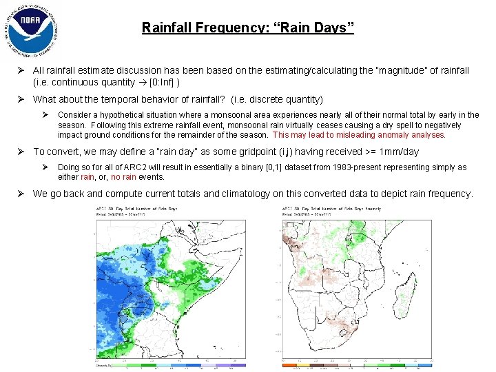
Rainfall Frequency: “Rain Days” Ø All rainfall estimate discussion has been based on the estimating/calculating the “magnitude” of rainfall (i. e. continuous quantity [0: Inf] ) Ø What about the temporal behavior of rainfall? (i. e. discrete quantity) Ø Consider a hypothetical situation where a monsoonal area experiences nearly all of their normal total by early in the season. Following this extreme rainfall event, monsoonal rain virtually ceases causing a dry spell to negatively impact ground conditions for the remainder of the season. This may lead to misleading anomaly analyses. Ø To convert, we may define a “rain day” as some gridpoint (i, j) having received >= 1 mm/day Ø Doing so for all of ARC 2 will result in essentially a binary [0, 1] dataset from 1983 -present representing simply as either rain, or, no rain events. Ø We go back and compute current totals and climatology on this converted data to depict rain frequency.

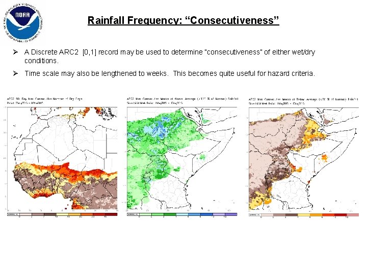
Rainfall Frequency: “Consecutiveness” Ø A Discrete ARC 2 [0, 1] record may be used to determine “consecutiveness” of either wet/dry conditions. Ø Time scale may also be lengthened to weeks. This becomes quite useful for hazard criteria.

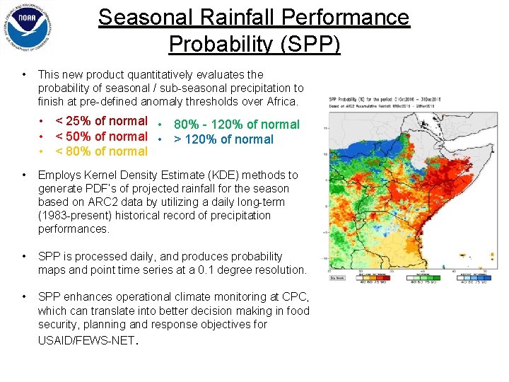
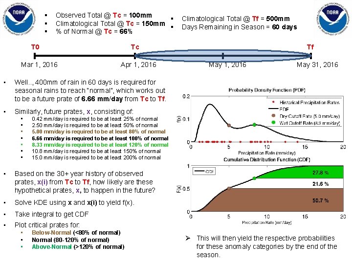
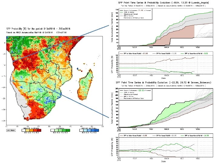
Seasonal Rainfall Performance Probability (SPP) • This new product quantitatively evaluates the probability of seasonal / sub-seasonal precipitation to finish at pre-defined anomaly thresholds over Africa. • < 25% of normal • 80% - 120% of normal • < 50% of normal • > 120% of normal • < 80% of normal • Employs Kernel Density Estimate (KDE) methods to generate PDF’s of projected rainfall for the season based on ARC 2 data by utilizing a daily long-term (1983 -present) historical record of precipitation performances. • SPP is processed daily, and produces probability maps and point time series at a 0. 1 degree resolution. • SPP enhances operational climate monitoring at CPC, which can translate into better decision making in food security, planning and response objectives for USAID/FEWS-NET.

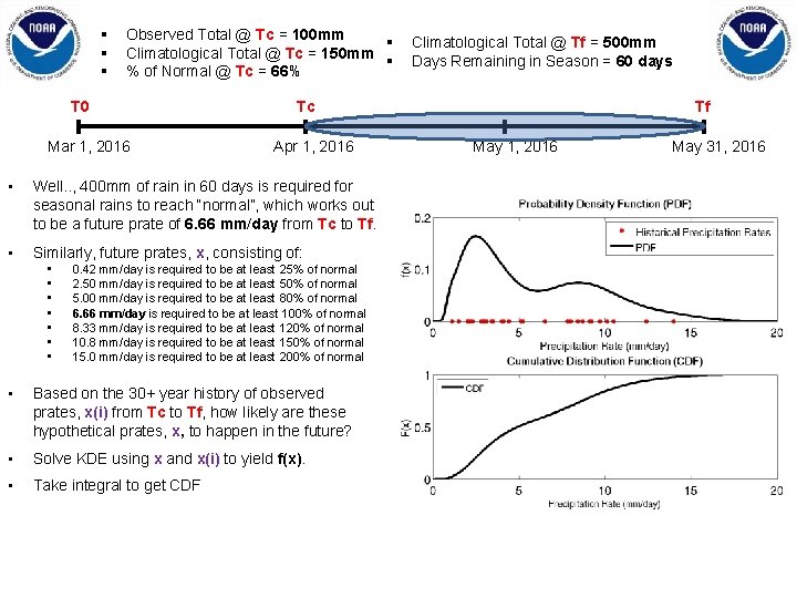
§ § § Observed Total @ Tc = 100 mm § Climatological Total @ Tc = 150 mm § % of Normal @ Tc = 66% T 0 Mar 1, 2016 Tc Apr 1, 2016 • Well. . , 400 mm of rain in 60 days is required for seasonal rains to reach “normal”, which works out to be a future prate of 6. 66 mm/day from Tc to Tf. • Similarly, future prates, x, consisting of: • • Climatological Total @ Tf = 500 mm Days Remaining in Season = 60 days 0. 42 mm/day is required to be at least 25% of normal 2. 50 mm/day is required to be at least 50% of normal 5. 00 mm/day is required to be at least 80% of normal 6. 66 mm/day is required to be at least 100% of normal 8. 33 mm/day is required to be at least 120% of normal 10. 8 mm/day is required to be at least 150% of normal 15. 0 mm/day is required to be at least 200% of normal • Based on the 30+ year history of observed prates, x(i) from Tc to Tf, how likely are these hypothetical prates, x, to happen in the future? • Solve KDE using x and x(i) to yield f(x). • Take integral to get CDF Tf May 1, 2016 May 31, 2016

§ § § Observed Total @ Tc = 100 mm § Climatological Total @ Tc = 150 mm § % of Normal @ Tc = 66% Tc T 0 Mar 1, 2016 Apr 1, 2016 • Well. . , 400 mm of rain in 60 days is required for seasonal rains to reach “normal”, which works out to be a future prate of 6. 66 mm/day from Tc to Tf. • Similarly, future prates, x, consisting of: • • Tf May 1, 2016 May 31, 2016 0. 42 mm/day is required to be at least 25% of normal 2. 50 mm/day is required to be at least 50% of normal 5. 00 mm/day is required to be at least 80% of normal 6. 66 mm/day is required to be at least 100% of normal 8. 33 mm/day is required to be at least 120% of normal 10. 8 mm/day is required to be at least 150% of normal 15. 0 mm/day is required to be at least 200% of normal • Based on the 30+ year history of observed prates, x(i) from Tc to Tf, how likely are these hypothetical prates, x, to happen in the future? • Solve KDE using x and x(i) to yield f(x). • Take integral to get CDF • Plot critical prates for: • • • Climatological Total @ Tf = 500 mm Days Remaining in Season = 60 days Below-Normal (<80% of normal) Normal (80 -120% of normal) Above-Normal (>120% of normal) Ø This will then yield the respective probabilities for these anomaly categories by the end of the season.

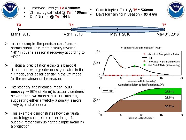
§ § § Observed Total @ Tc = 100 mm § Climatological Total @ Tc = 150 mm § % of Normal @ Tc = 66% T 0 Mar 1, 2016 Tc Apr 1, 2016 Ø In this example, the persistence of belownormal rainfall is climatologically favored (~51%) over a seasonal recovery according to ARC 2. Ø Historical precipitation exhibits a bimodal distribution, with greater density located in the 1 st mode, and lesser density in the 2 nd mode, for the remainder of the season. • Climatological Total @ Tf = 500 mm Days Remaining in Season = 60 days Interestingly, the historical mean (5. 83 mm/day 90% of Norm) is actually centered between the two modes in a PDF minima, suggesting either a wet/dry anomaly is more likely by end of season. Ø This example demonstrates how the rainfall climatology can create a more insightful outlook, rather than using the simple mean as a projection. Tf May 1, 2016 May 31, 2016

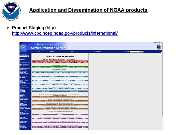
Application and Dissemination of NOAA products Ø Product Staging (http): http: //www. cpc. ncep. noaa. gov/products/international/

Questions / Comments …?