NOAA Satellite Conference 2015 POSTER 2 18 Using

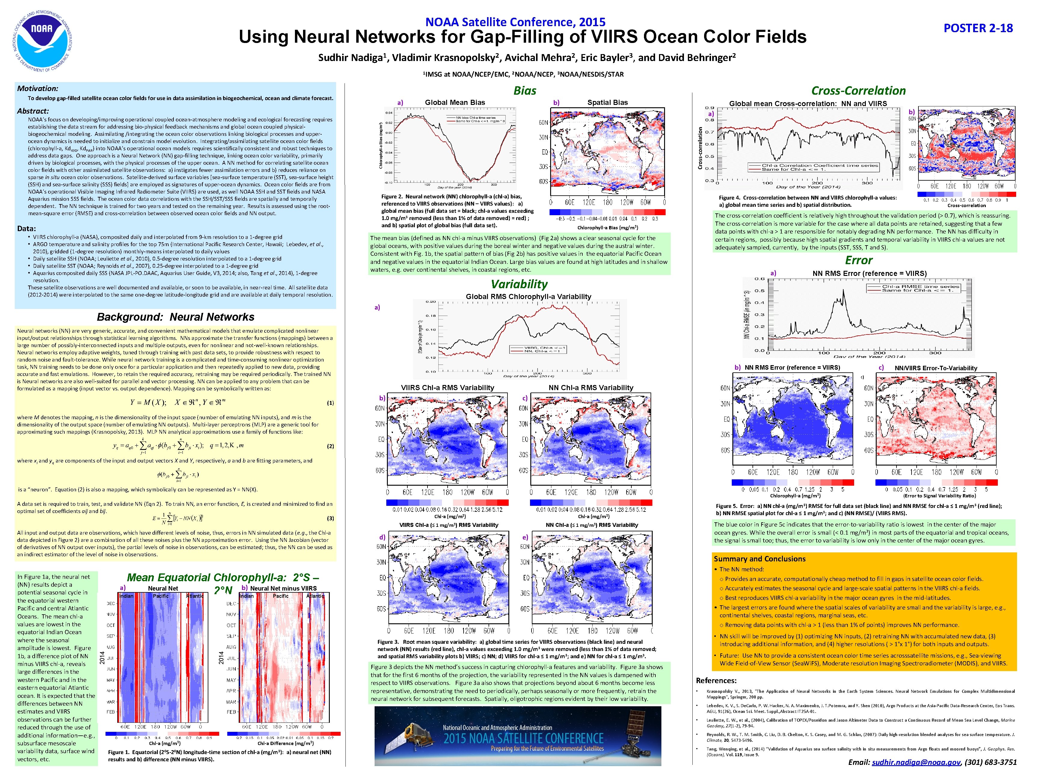
NOAA Satellite Conference, 2015 POSTER 2 -18 Using Neural Networks for Gap-Filling of VIIRS Ocean Color Fields Sudhir Nadiga 1, Vladimir Krasnopolsky 2, Avichal Mehra 2, Eric Bayler 3, and David Behringer 2 1 IMSG at NOAA/NCEP/EMC, 2 NOAA/NCEP, 3 NOAA/NESDIS/STAR Bias Motivation: To develop gap-filled satellite ocean color fields for use in data assimilation in biogeochemical, ocean and climate forecast. a) Abstract: Global mean Cross-correlation: NN and VIIRS b) a) Cross-correlation Figure 2. Neural network (NN) chlorophyll-a (chl-a) bias, referenced to VIIRS observations (NN – VIIRS values): a) global mean bias (full data set = black; chl-a values exceeding 1. 0 mg/m 3 removed (less than 1% of data removed) = red) ; and b) spatial plot of global bias (full data set). Data: • VIIRS chlorophyll-a (NASA), composited daily and interpolated from 9 -km resolution to a 1 -degree grid • ARGO temperature and salinity profiles for the top 75 m (International Pacific Research Center, Hawaii; Lebedev, et al. , 2010), gridded (1 -degree resolution) monthly-means interpolated to daily values • Daily satellite SSH (NOAA; Leuliette et al. , 2010), 0. 5 -degree resolution interpolated to a 1 -degree grid • Daily satellite SST (NOAA; Reynolds et al. , 2007), 0. 25 -degree interpolated to a 1 -degree grid • Aquarius composited daily SSS (NASA JPL-PO. DAAC, Aquarius User Guide, V 3, 2014; also, Tang et al. , 2014), 1 -degree resolution. These satellite observations are well documented and available, or soon to be available, in near-real time. All satellite data (2012 -2014) were interpolated to the same one-degree latitude-longitude grid and are available at daily temporal resolution. Spatial Bias Chlorophyll-a Bias (mg/m 3) NOAA’s focus on developing/improving operational coupled ocean-atmosphere modeling and ecological forecasting requires establishing the data stream for addressing bio-physical feedback mechanisms and global ocean coupled physicalbiogeochemical modeling. Assimilating /integrating the ocean color observations linking biological processes and upperocean dynamics is needed to initialize and constrain model evolution. Integrating/assimilating satellite ocean color fields (chlorophyll-a, Kd 490, Kd. PAR) into NOAA’s operational ocean models requires scientifically consistent and robust techniques to address data gaps. One approach is a Neural Network (NN) gap-filling technique, linking ocean color variability, primarily driven by biological processes, with the physical processes of the upper ocean. A NN method for correlating satellite ocean color fields with other assimilated satellite observations: a) instigates fewer assimilation errors and b) reduces reliance on sparse in situ ocean color observations. Satellite-derived surface variables [sea-surface temperature (SST), sea-surface height (SSH) and sea-surface salinity (SSS) fields] are employed as signatures of upper-ocean dynamics. Ocean color fields are from NOAA’s operational Visible Imaging Infrared Radiometer Suite (VIIRS) are used, as well NOAA SSH and SST fields and NASA Aquarius mission SSS fields. The ocean color data correlations with the SSH/SST/SSS fields are spatially and temporally dependent. The NN technique is trained for two years and tested on the remaining year. Results is assessed using the rootmean-square error (RMSE) and cross-correlation between observed ocean color fields and NN output. b) Global Mean Bias Cross-Correlation Figure 4. Cross-correlation between NN and VIIRS chlorophyll-a values: a) global mean time series and b) spatial distribution. Cross-correlation The cross-correlation coefficient is relatively high throughout the validation period (> 0. 7), which is reassuring. The cross-correlation is more variable for the case where all data points are retained, suggesting that a few data points with chl-a > 1 are responsible for notably degrading NN performance. The NN has difficulty in certain regions, possibly because high spatial gradients and temporal variability in VIIRS chl-a values are not adequately sampled, currently, by the inputs (SST, SSS, T and S). Chlorophyll-a Bias (mg/m 3) The mean bias (defined as NN chl-a minus VIIRS observations) (Fig 2 a) shows a clear seasonal cycle for the global oceans, with positive values during the boreal winter and negative values during the austral winter. Consistent with Fig. 1 b, the spatial pattern of bias (Fig 2 b) has positive values in the equatorial Pacific Ocean and negative values in the equatorial Indian Ocean. Large bias values are found at high latitudes and in shallow waters, e. g. over continental shelves, in coastal regions, etc. Error a) Variability NN RMS Error (reference = VIIRS) Global RMS Chlorophyll-a Variability (Cross-correlation) a) Background: Neural Networks Neural networks (NN) are very generic, accurate, and convenient mathematical models that emulate complicated nonlinear input/output relationships through statistical learning algorithms. NNs approximate the transfer functions (mappings) between a large number of possibly-interconnected inputs and multiple outputs, even for nonlinear and not-well-known relationships. Neural networks employ adaptive weights, tuned through training with past data sets, to provide robustness with respect to random noise and fault-tolerance. While neural network training is a complicated and time-consuming nonlinear optimization task, NN training needs to be done only once for a particular application and then repeatedly applied to new data, providing accurate and fast emulations. However, to retain the required accuracy, retraining may be required periodically. The trained NN is Neural networks are also well-suited for parallel and vector processing. NN can be applied to any problem that can be formulated as a mapping (input vector vs. output dependence). Mapping can be symbolically written as: (1) b) NN RMS Error (reference = VIIRS) c) NN/VIIRS Error-To-Variability c) VIIRS Chl-a RMS Variability b) NN Chl-a RMS Variability c) where M denotes the mapping, n is the dimensionality of the input space (number of emulating NN inputs), and m is the dimensionality of the output space (number of emulating NN outputs). Multi-layer perceptrons (MLP) are a generic tool for approximating such mappings (Krasnopolsky, 2013). MLP NN analytical approximations use a family of functions like: (2) where xi and yq are components of the input and output vectors X and Y, respectively, a and b are fitting parameters, and is a “neuron”. Equation (2) is also a mapping, which symbolically can be represented as Y = NN(X). A data set is required to train, test, and validate NN (Eqn 2). To train NN, an error function, E, is created and minimized to find an optimal set of coefficients aij and bij. (3) All input and output data are observations, which have different levels of noise, thus, errors in NN simulated data (e. g. , the Chl-a data depicted in Figure 2) are a combination of all these noises plus the NN approximation error. Using the NN Jacobian (vector of derivatives of NN output over inputs), the partial levels of noise in observations, can be estimated; thus, the NN can be used as an indirect estimator of the level of noise in observations. d) Chl-a (mg/m 3) VIIRS Chl-a (≤ 1 mg/m 3) RMS Variability NN Chl-a (≤ 1 mg/m 3) RMS Variability The blue color in Figure 5 c indicates that the error-to-variability ratio is lowest in the center of the major ocean gyres. While the overall error is small (< 0. 1 mg/m 3) in most parts of the equatorial and tropical oceans, the signal is small too; thus, the error to variability is low only in the center of the major ocean gyres. e) Summary and Conclusions • The NN method: o Provides an accurate, computationally cheap method to fill in gaps in satellite ocean color fields. o Accurately estimates the seasonal cycle and large-scale spatial patterns in the VIIRS chl-a fields. o Best reproduces VIIRS chl-a variability in the major ocean gyres in the mid-latitudes. • The largest errors are found where the spatial scales of variability are small and the variability is large, e. g. , continental shelves, coastal regions, marginal seas, etc. o Removing data points with chl-a > 1 (less than 1% of points) improves NN performance. • NN skill will be improved by (1) optimizing NN inputs, (2) retraining NN with accumulated new data, (3) introducing additional information, and (4) higher resolutions ( > 1°x 1°) for both inputs and outputs. Figure 3. Root mean square variability: a) global time series for VIIRS observations (black line) and neural network (NN) results (red line), chl-a values exceeding 1. 0 mg/m 3 were removed (less than 1% of data removed; and spatial RMS variability plots b) VIIRS; c) NN; d) VIIRS for chl-a ≤ 1 mg/m 3; and e) NN for chl-a ≤ 1 mg/m 3. 2014 Chl-a (mg/m 3) Figure 3 depicts the NN method’s success in capturing chlorophyll-a features and variability. Figure 3 a shows that for the first 6 months of the projection, the variability represented in the NN values is dampened with respect to VIIRS observations. Figure 3 a also shows that projections beyond about 6 months become less representative, demonstrating the need to periodically, perhaps seasonally or more frequently, retrain the neural network for subsequent forecasts. Spatially, oligotrophic regions evident by their low variability. Chl-a Difference (mg/m 3) Figure 1. Equatorial (20 S-20 N) longitude-time section of chl-a (mg/m 3): a) neural net (NN) results and b) difference (NN minus VIIRS). (Error to Signal Variability Ratio) Figure 5. Error: a) NN chl-a (mg/m 3) RMSE for full data set (black line) and NN RMSE for chl-a ≤ 1 mg/m 3 (red line); b) NN RMSE spatial plot for chl-a ≤ 1 mg/m 3; and c) (NN RMSE)/ (VIIRS RMS). Mean Equatorial Chlorophyll-a: 2°S – a) b) Neural Net minus VIIRS Neural Net 2°N Indian Pacific Atlantic 2014 In Figure 1 a, the neural net (NN) results depict a potential seasonal cycle in the equatorial western Pacific and central Atlantic Oceans. The mean chl-a values are lowest in the equatorial Indian Ocean where the seasonal amplitude is lowest. Figure 1 b, a difference plot of NN minus VIIRS chl-a, reveals large differences in the western Pacific and in the eastern equatorial Atlantic ocean. It is expected that the differences between NN estimates and VIIRS observations can be further reduced through the use of additional information—e. g. , subsurface mesoscale variability data, surface wind vectors, etc. Chlorophyll-a (mg/m 3) • Future: Use NN to provide a consistent ocean color time series acrosssatellite missions, e. g. , Sea-viewing Wide Field-of-View Sensor (Sea. Wi. FS), Moderate resolution Imaging Spectroradiometer (MODIS), and VIIRS. References: • Krasnopolsky V. , 2013, "The Application of Neural Networks in the Earth System Sciences. Neural Network Emulations for Complex Multidimensional Mappings", Springer, 200 pp. • Lebedev, K. V. , S. De. Carlo, P. W. Hacker, N. A. Maximenko, J. T. Potemra, and Y. Shen (2010), Argo Products at the Asia-Pacific Data-Research Center, Eos Trans. AGU, 91(26), Ocean Sci. Meet. Suppl. , Abstract IT 25 A-01. • Leuliette, E. W. , et al. , (2004), Calibration of TOPEX/Poseidon and Jason Altimeter Data to Construct a Continuous Record of Mean Sea Level Change, Marine Geodesy, 27(1 -2), 79 -94 • Reynolds, R. W. , T. M. Smith, C. Liu, D. B. Chelton, K. S. Casey, and M. G. Schlax, (2007): Daily high-resolution blended analyses for sea surface temperature. J. Climate, 20, 5473 -5496. • Tang, Wenqing, et al. , (2014) “Validation of Aquarius sea surface salinity with in situ measurements from Argo floats and moored buoys”, J. Geophys. Res. (Oceans), Vol. 119, Issue 9. Email: sudhir. nadiga@noaa. gov, (301) 683 -3751