COST OF EQUITY CAPITAL Outline Introduction The Dividend

COST OF EQUITY CAPITAL

Outline • Introduction • The Dividend Discount Model • CAPM to derive the cost of equity capital

Dividend Discount Model: basics The basics for deriving the cost of equity capital could be summed up in the following statement: The equity value is given by the present value of expected future dividends at an appropriate risk-adjusted cost of capital

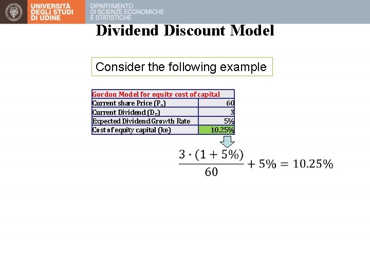
Dividend Discount Model • The equity value can be derived as follows: • Which can be reduced to the following form: • Finally, we can extract the cost of capital:

Dividend Discount Model Consider the following example Gordon Model for equity cost of capital Current share Price (P 0) 60 Current Dividend (D 0) 3 Expected Dividend Growth Rate 5% Cost of equity capital (ke) 10. 25%

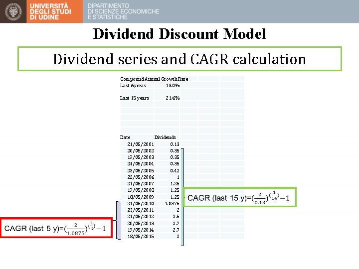
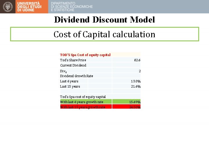
Dividend Discount Model • Example: Tod’s Spa • Let consider the dividend series over the last 15 years • Calculate the Compound Annual Growth Rate (CAGR) for the last 6 and 15 years respectively • Apply the Gordon Model for deriving the cost of equity capital

Dividend Discount Model Dividend series and CAGR calculation Compound Annual Growth Rate Last 6 yeras 13. 0% Last 15 years 21. 6% Date Dividends 21/05/2001 0. 13 20/05/2002 0. 35 19/05/2003 0. 35 24/05/2004 0. 35 23/05/2005 0. 42 22/05/2006 1 21/05/2007 1. 25 19/05/2008 1. 25 18/05/2009 1. 25 24/05/2010 1. 0875 23/05/2011 2 21/05/2012 2. 5 20/05/2013 2. 7 19/05/2014 2. 7 18/05/2015 2

Dividend Discount Model Cost of Capital calculation TOD'S Spa Cost of equity capital Tod's Share Price Current Dividend Div 0 Dividend Growth Rate Last 6 years Last 15 years Tod's Spa cost of equity capital With last 6 years growth rate With last 15 years growth rate 82. 6 2 13. 0% 21. 6% 15. 69% 24. 50%

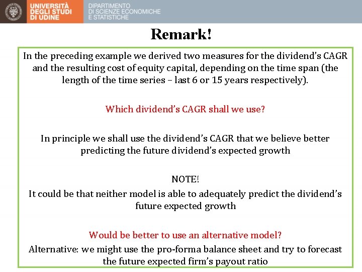
Remark! In the preceding example we derived two measures for the dividend’s CAGR and the resulting cost of equity capital, depending on the time span (the length of the time series – last 6 or 15 years respectively). Which dividend’s CAGR shall we use? In principle we shall use the dividend’s CAGR that we believe better predicting the future dividend’s expected growth NOTE! It could be that neither model is able to adequately predict the dividend’s future expected growth Would be better to use an alternative model? Alternative: we might use the pro-forma balance sheet and try to forecast the future expected firm’s payout ratio

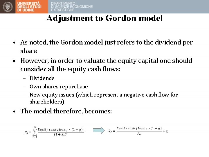
Adjustment to Gordon model • As noted, the Gordon model just refers to the dividend per share • However, in order to valuate the equity capital one should consider all the equity cash flows: – Dividends – Own shares repurchase – New equity issues (which represent a negative cash flow for shareholders) • The model therefore, becomes:

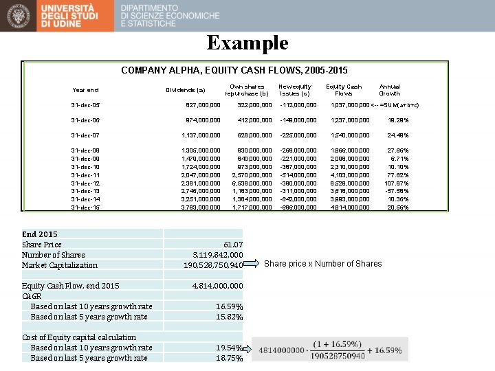
Example COMPANY ALPHA, EQUITY CASH FLOWS, 2005 -2015 Year end Own shares repurchase (b) Dividends (a) New equity issues (c) Equity Cash Flows Annual Growth 31 -dec-05 827, 000 322, 000 -112, 000 1, 037, 000 <-- =SUM(a+b+c) 31 -dec-06 974, 000 412, 000 -149, 000 1, 237, 000 19. 29% 31 -dec-07 1, 137, 000 628, 000 -225, 000 1, 540, 000 24. 49% 31 -dec-08 31 -dec-09 31 -dec-10 31 -dec-11 31 -dec-12 31 -dec-13 31 -dec-14 31 -dec-15 1, 305, 000 1, 479, 000 1, 724, 000 2, 047, 000 2, 381, 000 2, 746, 000 3, 251, 000 3, 793, 000 930, 000 840, 000 973, 000 2, 570, 000 6, 538, 000 1, 183, 000 1, 384, 000 1, 717, 000 -269, 000 -221, 000 -387, 000 -514, 000 -390, 000 -311, 000 -642, 000 -696, 000 1, 966, 000 2, 098, 000 2, 310, 000 4, 103, 000 8, 529, 000 3, 618, 000 3, 993, 000 4, 814, 000 27. 66% 6. 71% 10. 10% 77. 62% 107. 87% -57. 58% 10. 36% 20. 56% End 2015 Share Price Number of Shares Market Capitalization Equity Cash Flow, end 2015 CAGR Based on last 10 years growth rate Based on last 5 years growth rate Cost of Equity capital calculation Based on last 10 years growth rate Based on last 5 years growth rate 61. 07 3, 119, 842, 000 190, 528, 750, 940 Share price x Number of Shares 4, 814, 000 16. 59% 15. 82% 19. 54% 18. 75%

Using the CAPM for deriving the cost of equity capital • The CAPM is the most widely used model for the cost of equity capital calculation • As known the model derives the cost of equity capital from the covariance with market returns • In order to apply the CAPM we need to know: – The risk free rate – The equity beta – The market return

The equity beta • Three possible approaches for calculating equity betas: – Regression beta – Bottom-up approach (based on comparables) – Accounting beta

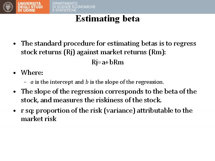
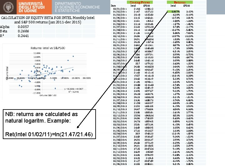
Estimating beta • The standard procedure for estimating betas is to regress stock returns (Rj) against market returns (Rm): Rj=a+b. Rm • Where: – a is the intercept and b is the slope of the regression. • The slope of the regression corresponds to the beta of the stock, and measures the riskiness of the stock. • r sq: proportion of the risk (variance) attributable to the market risk

How to estimate betas? • Decide on estimation period – Long term vs short term horizon trade off – Long periods expected to provide more reliable. Firm changes? – What about short term periods? • Decide on a return interval (daly, weekly. . ) • Estimating returns • Choose a market index

Closing Prices CALCULATION OF EQUITY BETA FOR INTEL Monthly Intel and S&P 500 returns (jan 2011 -dec 2015) Alpha 0. 0057 Beta 0. 2686 R 2 0. 2441 NB: returns are calculated as natural logaritm. Example: Ret(Intel 01/02/11)=ln(21. 47/21. 46) Date 03/01/2011 01/02/2011 01/03/2011 01/04/2011 02/05/2011 01/06/2011 01/07/2011 01/08/2011 01/09/2011 03/10/2011 01/11/2011 01/12/2011 03/01/2012 01/02/2012 01/03/2012 02/04/2012 01/05/2012 01/06/2012 02/07/2012 01/08/2012 04/09/2012 01/10/2012 01/11/2012 03/12/2012 02/01/2013 01/02/2013 01/03/2013 01/04/2013 01/05/2013 03/06/2013 01/07/2013 01/08/2013 03/09/2013 01/10/2013 01/11/2013 02/12/2013 02/01/2014 03/02/2014 03/03/2014 01/04/2014 01/05/2014 02/06/2014 01/07/2014 01/08/2014 02/09/2014 01/10/2014 03/11/2014 01/12/2014 02/01/2015 02/02/2015 02/03/2015 01/04/2015 Intel 21. 46 21. 47 20. 18 23. 15 22. 51 22. 16 22. 33 20. 13 21. 34 24. 54 24. 91 24. 25 26. 42 26. 88 28. 12 28. 4 25. 84 26. 65 25. 7 24. 83 22. 66 21. 63 19. 57 20. 62 21. 04 20. 88 21. 84 23. 95 24. 28 24. 23 23. 34 21. 98 22. 92 24. 47 23. 84 25. 96 24. 54 24. 76 25. 81 26. 69 27. 32 30. 9 33. 89 34. 92 34. 82 34. 01 37. 25 36. 29 33. 04 33. 25 31. 27 32. 55 SP 500 1286. 12 1327. 22 1325. 83 1363. 61 1345. 2 1320. 64 1292. 28 1218. 89 1131. 42 1253. 3 1246. 96 1257. 6 1312. 41 1365. 68 1408. 47 1397. 91 1310. 33 1362. 16 1379. 32 1406. 58 1440. 67 1412. 16 1416. 18 1426. 19 1498. 11 1514. 68 1569. 19 1597. 57 1630. 74 1606. 28 1685. 73 1632. 97 1681. 55 1756. 54 1805. 81 1848. 36 1782. 59 1859. 45 1872. 34 1883. 95 1923. 57 1960. 23 1930. 67 2003. 37 1972. 29 2018. 05 2067. 56 2058. 9 1994. 99 2104. 5 2067. 89 2085. 51 Returns Intel 0. 047% -6. 20% 13. 73% -2. 80% -1. 57% 0. 76% -10. 37% 5. 84% 13. 97% 1. 50% -2. 69% 8. 57% 1. 73% 4. 51% 0. 99% -9. 45% 3. 09% -3. 63% -3. 44% -9. 15% -4. 65% -10. 01% 5. 23% 2. 02% -0. 76% 4. 50% 9. 22% 1. 37% -0. 21% -3. 74% -6. 00% 4. 19% 6. 54% -2. 61% 8. 52% -5. 63% 0. 89% 4. 15% 3. 35% 2. 33% 12. 31% 9. 24% 2. 99% -0. 29% -2. 35% 9. 10% -2. 61% -9. 38% 0. 63% -6. 14% 4. 01% SP 500 3. 15% -0. 10% 2. 81% -1. 36% -1. 84% -2. 17% -5. 85% -7. 45% 10. 23% -0. 51% 0. 85% 4. 27% 3. 98% 3. 09% -0. 75% -6. 47% 3. 88% 1. 25% 1. 96% 2. 39% -2. 00% 0. 28% 0. 70% 4. 92% 1. 10% 3. 54% 1. 79% 2. 06% -1. 51% 4. 83% -3. 18% 2. 93% 4. 36% 2. 77% 2. 33% -3. 62% 4. 22% 0. 69% 0. 62% 2. 08% 1. 89% -1. 52% 3. 70% -1. 56% 2. 29% 2. 42% -0. 42% -3. 15% 5. 34% -1. 75% 0. 85%

Determinants of betas? • Industry effects – How should you expect betas of cyclical companies to be? – And those of companies producing discretionary goods? • Operating leverage • Financial leverage – We distinguish • Beta levered • Beta unlevered

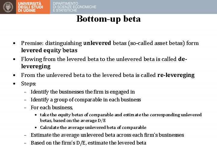
Bottom-up beta • Premise: distinguishing unlevered betas (so-called asset betas) form levered equity betas • Flowing from the levered beta to the unlevered beta is called delevereging • From the unlevered beta to the levered beta is called re-levereging • Steps: – Identify the businesses the firm is engaged in – Identify a group of comparable in each business – For each business, • take the equity betas of comparable and estimate the corresponding unlevered betas, based on the average D/E • Calculate the average unlevered beta of comparable – Estimate the average unlevered beta across each firm’s businesses – Based on the firm’s D/E, estimate the levered beta

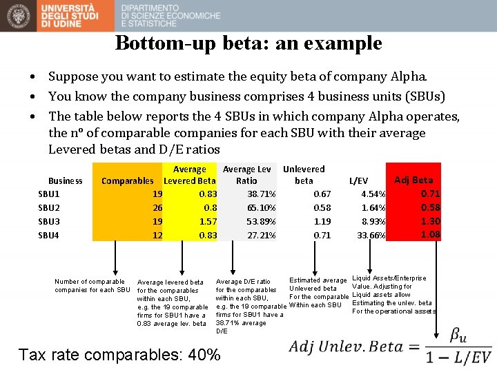
Bottom-up beta: an example • Suppose you want to estimate the equity beta of company Alpha. • You know the company business comprises 4 business units (SBUs) • The table below reports the 4 SBUs in which company Alpha operates, the n° of comparable companies for each SBU with their average Levered betas and D/E ratios Business SBU 1 SBU 2 SBU 3 SBU 4 Average Lev Unlevered Comparables Levered Beta Ratio beta 19 0. 83 38. 71% 0. 67 26 0. 8 65. 10% 0. 58 19 1. 57 53. 89% 1. 19 12 0. 83 27. 21% 0. 71 Number of comparable companies for each SBU Average levered beta for the comparables within each SBU, e. g. the 19 comparable firms for SBU 1 have a 0. 83 average lev. beta Estimated average Average D/E ratio Unlevered beta for the comparables For the comparable within each SBU, e. g. the 19 comparable Within each SBU firms for SBU 1 have a 38. 71% average D/E Tax rate comparables: 40% Adj Beta L/EV 0. 71 4. 54% 0. 58 1. 64% 1. 30 8. 93% 1. 08 33. 66% Liquid Assets/Enterprise Value. Adjusting for Liquid assets allow Estimating the unlev. beta For the operational assets

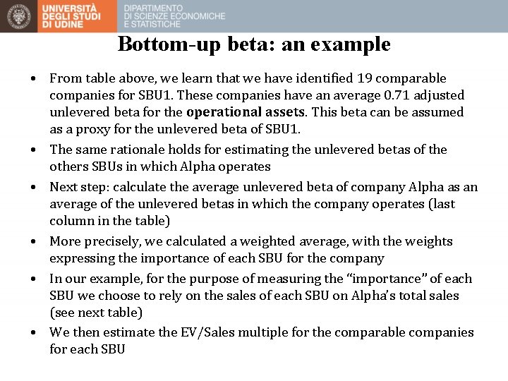
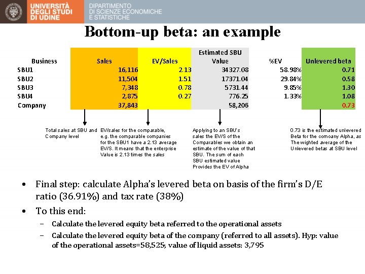
Bottom-up beta: an example • From table above, we learn that we have identified 19 comparable companies for SBU 1. These companies have an average 0. 71 adjusted unlevered beta for the operational assets. This beta can be assumed as a proxy for the unlevered beta of SBU 1. • The same rationale holds for estimating the unlevered betas of the others SBUs in which Alpha operates • Next step: calculate the average unlevered beta of company Alpha as an average of the unlevered betas in which the company operates (last column in the table) • More precisely, we calculated a weighted average, with the weights expressing the importance of each SBU for the company • In our example, for the purpose of measuring the “importance” of each SBU we choose to rely on the sales of each SBU on Alpha’s total sales (see next table) • We then estimate the EV/Sales multiple for the comparable companies for each SBU

Bottom-up beta: an example Business SBU 1 SBU 2 SBU 3 SBU 4 Company Sales EV/Sales 16, 116 11, 504 7, 348 2, 875 37, 843 Total sales at SBU and EV/sales for the comparable, Company level e. g. the comparable companies for the SBU 1 have a 2. 13 average EV/S. It means that the enterprise Value is 2. 13 times the sales 2. 13 1. 51 0. 78 0. 27 Estimated SBU Value 34327. 08 17371. 04 5731. 44 776. 25 58, 206 Applying to an SBU’s sales the EV/S of the Comparables we obtain an estimate of the value of that SBU. The sum of each SBU estimated value Provides the EV of Alpha %EV Unlevered beta 58. 98% 0. 71 29. 84% 0. 58 9. 85% 1. 30 1. 33% 1. 08 0. 73 is the estimated unlevered Beta for the comoany Alpha, as The wighted average of the Unlevered betas at SBU level • Final step: calculate Alpha’s levered beta on basis of the firm’s D/E ratio (36. 91%) and tax rate (38%) • To this end: – Calculate the levered equity beta referred to the operational assets – Calculate the levered equity beta of the company (referred to all assets). Hyp: value of the operational assets=58, 525; value of liquid assets: 3, 795

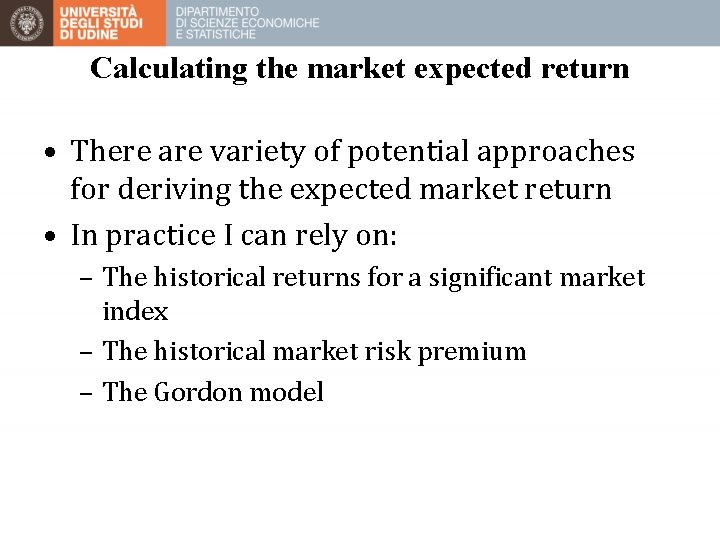
Calculating the market expected return • There are variety of potential approaches for deriving the expected market return • In practice I can rely on: – The historical returns for a significant market index – The historical market risk premium – The Gordon model

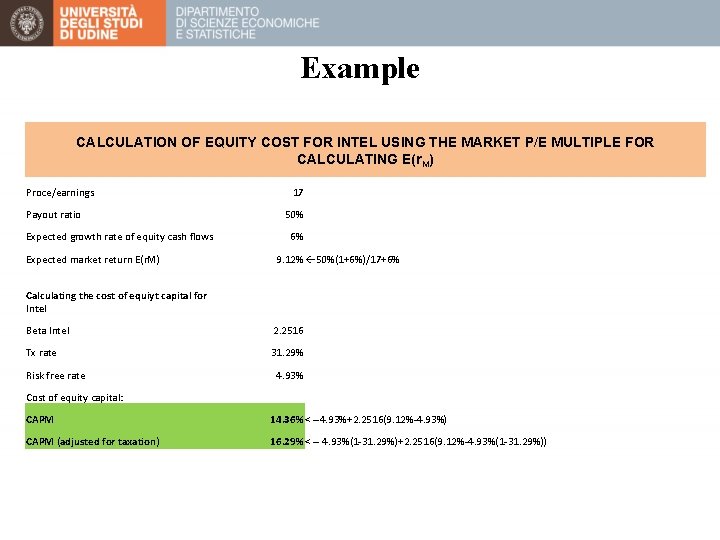
Calculating the market expected return • If we don’t believe that market expected returns are appropriately represented by past time series, we can rely on current market data to directly extract them • The Gordon Model is useful for accomplishing that task • Recall the following equation: • Such an equation holds for the market portfolio as well: • Div 0, P 0, and g are the current dividend, the current price and the growth rate for the market portfolio. Supposing that the firms distributes a portion b of its earnings (EPS 0) as dividend we can rewrite: • Where P 0/ EPS 0 is the price-to-earnings ratio of the market

Example CALCULATION OF EQUITY COST FOR INTEL USING THE MARKET P/E MULTIPLE FOR CALCULATING E(r. M) Proce/earnings Payout ratio Expected growth rate of equity cash flows Expected market return E(r. M) 17 50% 6% 9. 12% 50%(1+6%)/17+6% Calculating the cost of equiyt capital for Intel Beta Intel 2. 2516 Tx rate 31. 29% Risk free rate 4. 93% Cost of equity capital: CAPM 14. 36% < --4. 93%+2. 2516(9. 12%-4. 93%) CAPM (adjusted for taxation) 16. 29% < -- 4. 93%(1 -31. 29%)+2. 2516(9. 12%-4. 93%(1 -31. 29%))

THE RISK OF DEBT

The risk of debt • Two main sources of risk (but not exhaustive): – Default risk – Recovery risk • Different to the equity the assessment of the risk of debt is much more focused on the specific risk • Why?

Rating • On debt markets the creditworthiness of issuers is often assessed by specialized agencies (rating agencies ) whose judgements represent the opinion of the agency on the ability of the issuer of meeting its commitments • Particularly useful for: – Intermediaries – Issuers – Investors

Ratings • Periodically revised • Assessments can change (upgrades o downgrades) due to: – Changes in macro-variables – Indistry-related dynamics or trends – Specific factors (at company or issue level) • Widely used jargons (anticipating possible changes to the firm’s/issue rating in the short-term) – Outlook (positive, negative, stable, developing) – Credit-watch

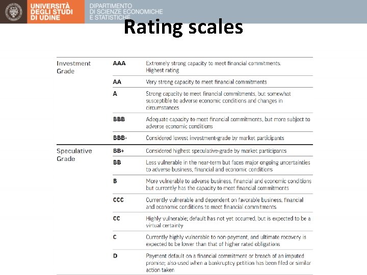
Rating scales

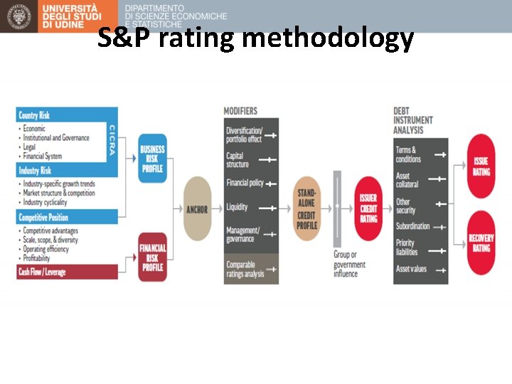
S&P rating methodology

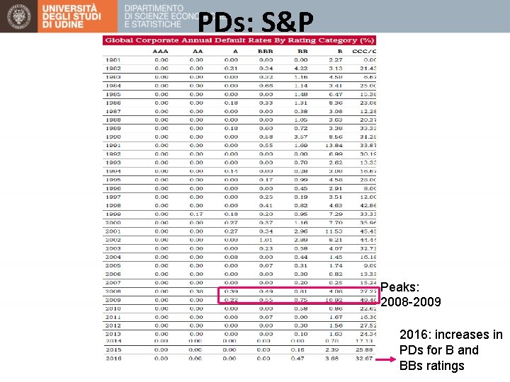
PDs: S&P Peaks: 2008 -2009 2016: increases in PDs for B and BBs ratings

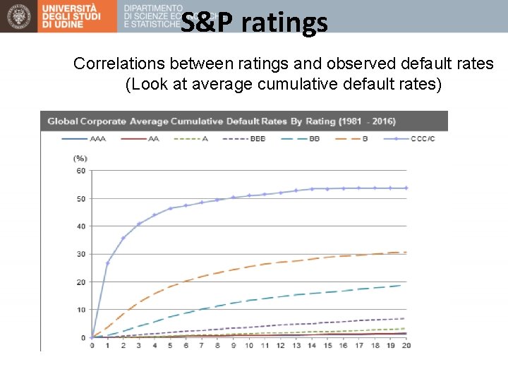
S&P ratings Correlations between ratings and observed default rates (Look at average cumulative default rates)

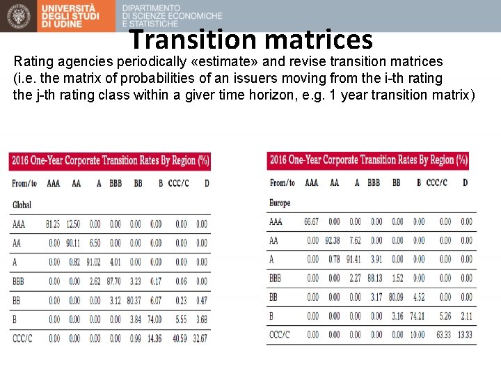
Transition matrices Rating agencies periodically «estimate» and revise transition matrices (i. e. the matrix of probabilities of an issuers moving from the i-th rating the j-th rating class within a giver time horizon, e. g. 1 year transition matrix)

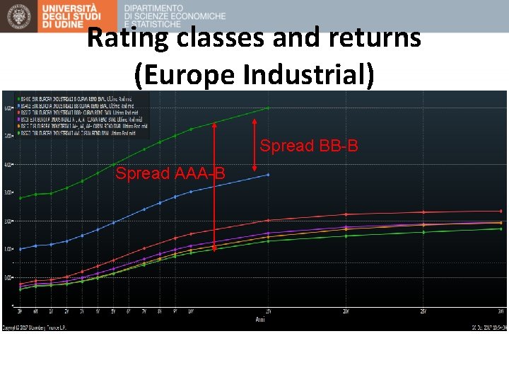
Rating classes and returns (Europe Industrial) Spread BB-B Spread AAA-B

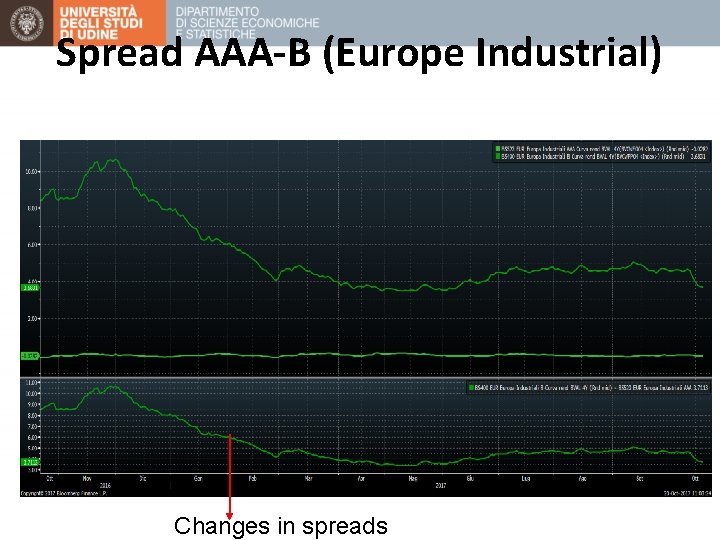
Spread AAA-B (Europe Industrial) Changes in spreads

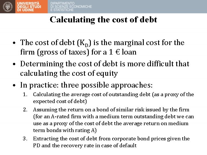
Calculating the cost of debt • The cost of debt (KD) is the marginal cost for the firm (gross of taxes) for a 1 € loan • Determining the cost of debt is more difficult that calculating the cost of equity • In practice: three possible approaches: 1. Calculating the average cost of outstanding debt (as a proxy of the expected cost of debt) 2. Assuming the return on a bond of similar risk issued by the firm (for an A-rated firm with a medium term outstanding debt we can use as a proxy of the cost of debt the average return on medium term bonds with rating A) 3. Extracting the cost of debt from corporate bond prices given the PD and the recovery rate in case of default

Calculating the cost of debt Methods 1 and 2 are easy to apply. Although they are not always so rigorous on a theoretical point of view, the estimation errors they are exposed to do not invalidate their advantages Method 3 is more rigorous on a theoretical point of view…but more difficult to apply! It is not always worth the effort

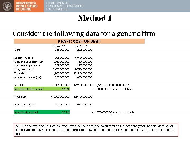
Method 1 Consider the following data for a generic firm KRAFT: COST OF DEBT Cash 31/12/2015 316, 000 31/12/2014 282, 000 Short term debt Maturing Long term debt Debt vs company alfa Long term debt Total debt Interest expenses (net) 805, 000 1, 268, 000 652, 000 8, 475, 000 11, 200, 000 636, 000 1, 818, 000 750, 000 227, 000 9, 723, 000 12, 518, 000 666, 000 Net debt Net interest rate on debt 10, 884, 000 5. 50% 12, 236, 000< -- (12518000000 -282000000) < -- 636000000/(average net debt) Total debt 11, 200, 000 12, 518, 000 679, 000 633, 000 Interest expenses Interest rate on debt 5. 73% < -- 679000000/(average total debt) 5. 5% is the average net interest rate payed by the company calculated on the net debt (total financial debt net of cash balances). 5. 73% is the average interest rate payed on total debt. Both can be used as proxies of the cost of debt

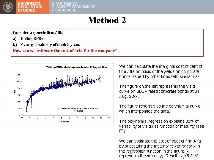
Method 2 Consider a generic firm Alfa. a) Rating BBB+ b) Average maturity of debt: 5 years How can we estimate the cost of debt for the company? We can calculate the marginal cost of debt of firm Alfa on basis of the yields on corporate bonds issued by other firms with similar risk The figure on the left represents the yield curve on BBB+ rated corporate bonds at 31 Aug. 20 xx. The figure reports also the polynomial curve which interpolates the data. The polynomial regression explains 85% of variability of yields as function of maturity (see R 2) We can estimate the cost of debt of firm Alfa by substituting the maturity (5 years) for x in the regression function in the figure (x represents the maturity). Result: KD=5. 31%

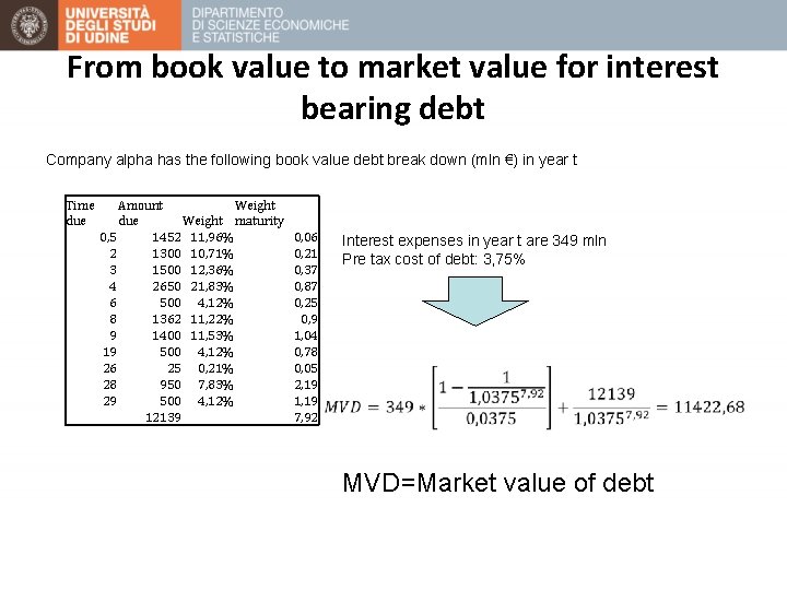
From book value to market value for interest bearing debt Company alpha has the following book value debt break down (mln €) in year t Time due Amount Weight due Weight maturity 0, 5 1452 11, 96% 2 1300 10, 71% 3 1500 12, 36% 4 2650 21, 83% 6 500 4, 12% 8 1362 11, 22% 9 1400 11, 53% 19 500 4, 12% 26 25 0, 21% 28 950 7, 83% 29 500 4, 12% 12139 0, 06 0, 21 0, 37 0, 87 0, 25 0, 9 1, 04 0, 78 0, 05 2, 19 1, 19 7, 92 Interest expenses in year t are 349 mln Pre tax cost of debt: 3, 75% MVD=Market value of debt