
Chapter 12 Estimating the Cost of Capital Copyright














- Slides: 73
Chapter 12 Estimating the Cost of Capital Copyright © 2017 Pearson Education, Ltd. All rights reserved. 12 -
12. 1 The Cost of Capital • The cost of capital is an opportunity cost concept. The required return on an investment has to match the return on an equivalent investment in the capital market. • If you believe the CAPM, equivalent investments should have the same beta. • It is also desirable for the investment and its capital market equivalent to have the same maturity. Copyright © 2017 Pearson Education, Ltd. All rights reserved. 12 -7
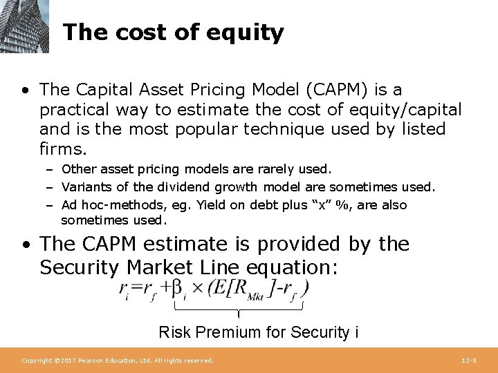
The cost of equity • The Capital Asset Pricing Model (CAPM) is a practical way to estimate the cost of equity/capital and is the most popular technique used by listed firms. – Other asset pricing models are rarely used. – Variants of the dividend growth model are sometimes used. – Ad hoc-methods, eg. Yield on debt plus “x” %, are also sometimes used. • The CAPM estimate is provided by the Security Market Line equation: Risk Premium for Security i Copyright © 2017 Pearson Education, Ltd. All rights reserved. 12 -8
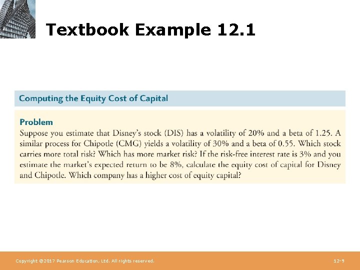
Textbook Example 12. 1 Copyright © 2017 Pearson Education, Ltd. All rights reserved. 12 -9
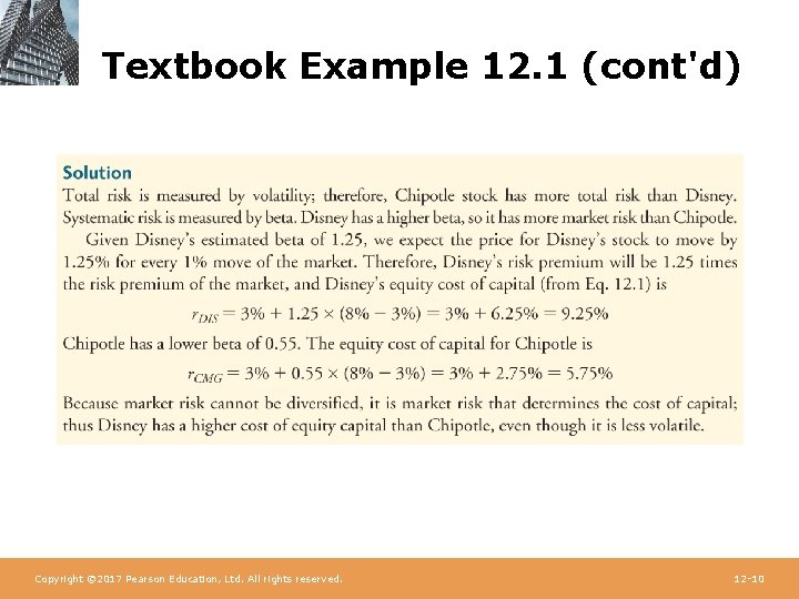
Textbook Example 12. 1 (cont'd) Copyright © 2017 Pearson Education, Ltd. All rights reserved. 12 -10
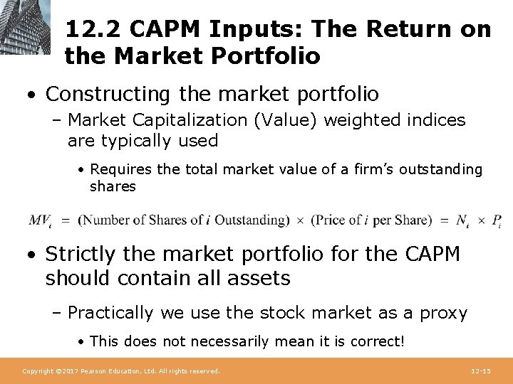
12. 2 CAPM Inputs: The Return on the Market Portfolio • Constructing the market portfolio – Market Capitalization (Value) weighted indices are typically used • Requires the total market value of a firm’s outstanding shares • Strictly the market portfolio for the CAPM should contain all assets – Practically we use the stock market as a proxy • This does not necessarily mean it is correct! Copyright © 2017 Pearson Education, Ltd. All rights reserved. 12 -15
12. 2 The Market Portfolio (cont’d) • Value-Weighted Portfolio – A portfolio in which each security is held in proportion to its market capitalization Copyright © 2017 Pearson Education, Ltd. All rights reserved. 12 -16
Value-Weighted Portfolios • A value-weighted portfolio is an equalownership portfolio; it contains an equal fraction of the total number of shares outstanding of each security in the portfolio. – Eg. Investing 1% of total market value, buy 1% of shares on issue for each firm. • Result: A relatively Passive Portfolio – A portfolio that is not rebalanced in response to price changes Copyright © 2017 Pearson Education, Ltd. All rights reserved. 12 -17
Investing in a Market Index • Index funds – mutual funds that invest in the S&P 500, the Wilshire 5000, or some other index. • Exchange-traded funds (ETFs) – trade directly on an exchange and represent ownership in a portfolio of stocks. – Example: SPDRS (Standard and Poor’s Depository Receipts) represent ownership in the S&P 500 Copyright © 2017 Pearson Education, Ltd. All rights reserved. 12 -19
12. 2 The Market Portfolio (cont’d) • In Australia the main indices are: – The All Ordinaries Index (500 largest companies) – S&P/ASX 200 Index (Largest 200) • Commonly viewed as the investment universe for fund managers – There is also an S&P/ASX 200 Franking Credit Adjusted Total Return Index – There also Accumulation Indices that allow for growth from the reinvestment of dividends Copyright © 2017 Pearson Education, Ltd. All rights reserved. 12 -20
The Market Risk Premium • Determining the Risk-Free Rate – The yield on U. S. Treasury securities – Surveys suggest most practitioners use 10 - to 30 -year treasuries – 30 Day Treasury Notes are the closest thing to risk free, but don’t match typical investment lives. • The Historical Risk Premium – Estimate the risk premium (E[RMkt]-rf) using the historical average excess return of the market over the risk-free interest rate Copyright © 2017 Pearson Education, Ltd. All rights reserved. 12 -21
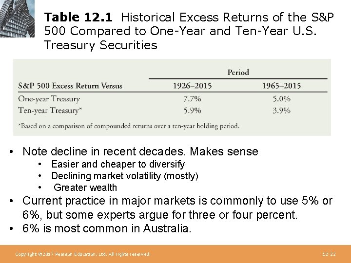
Table 12. 1 Historical Excess Returns of the S&P 500 Compared to One-Year and Ten-Year U. S. Treasury Securities • Note decline in recent decades. Makes sense • Easier and cheaper to diversify • Declining market volatility (mostly) • Greater wealth • Current practice in major markets is commonly to use 5% or 6%, but some experts argue for three or four percent. • 6% is most common in Australia. Copyright © 2017 Pearson Education, Ltd. All rights reserved. 12 -22
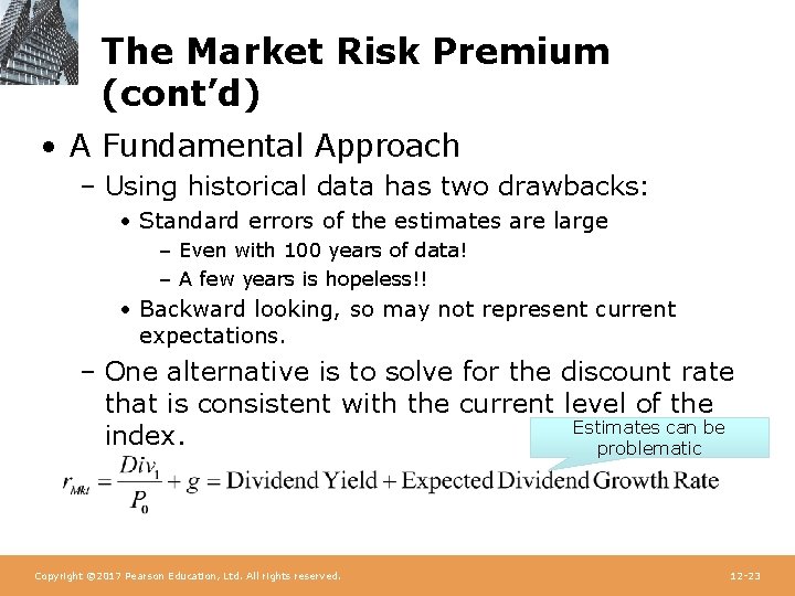
The Market Risk Premium (cont’d) • A Fundamental Approach – Using historical data has two drawbacks: • Standard errors of the estimates are large – Even with 100 years of data! – A few years is hopeless!! • Backward looking, so may not represent current expectations. – One alternative is to solve for the discount rate that is consistent with the current level of the Estimates can be index. problematic Copyright © 2017 Pearson Education, Ltd. All rights reserved. 12 -23
12. 3 Beta Estimation • Estimating Beta from Historical Returns – Recall, beta is the expected percent change in the excess return of the security for a 1% change in the excess return of the market portfolio. – Consider Cisco Systems stock and how it changes with the market portfolio. Copyright © 2017 Pearson Education, Ltd. All rights reserved. 12 -24
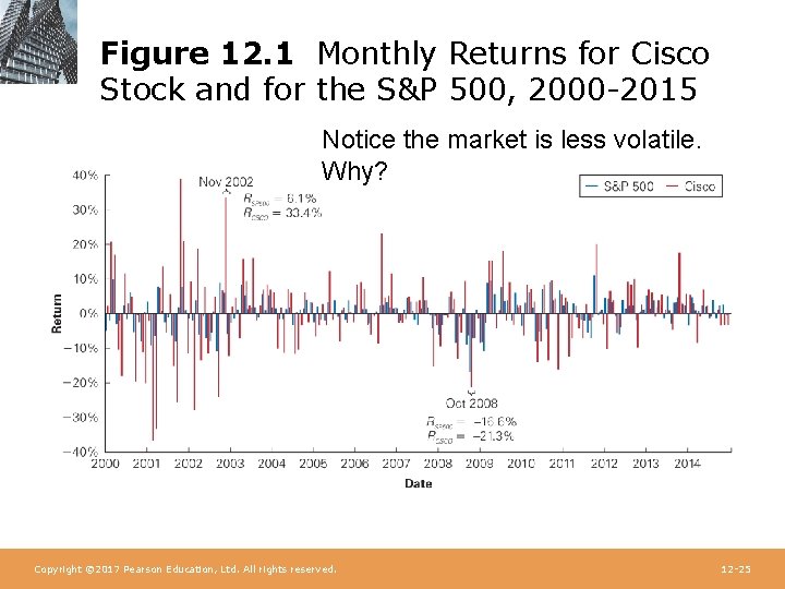
Figure 12. 1 Monthly Returns for Cisco Stock and for the S&P 500, 2000 -2015 Notice the market is less volatile. Why? Copyright © 2017 Pearson Education, Ltd. All rights reserved. 12 -25
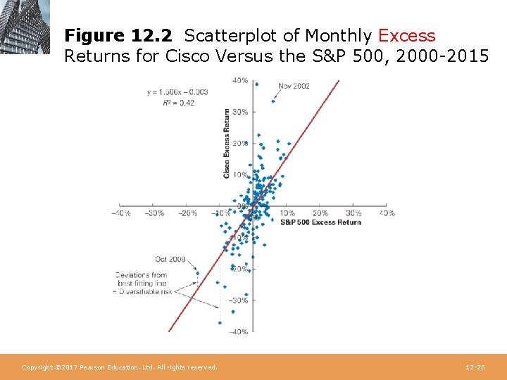
Figure 12. 2 Scatterplot of Monthly Excess Returns for Cisco Versus the S&P 500, 2000 -2015 Copyright © 2017 Pearson Education, Ltd. All rights reserved. 12 -26
12. 3 Beta Estimation (cont'd) • Estimating Beta from Historical Returns – As the scatterplot on the previous slide shows, Cisco tends to be up when the market is up, and vice versa. – We can see that a 10% change in the market’s return corresponds to about a 15% change in Cisco’s return. • Thus, Cisco’s return moves one and a half times the overall market, so Cisco’s beta is about 1. 5 Copyright © 2017 Pearson Education, Ltd. All rights reserved. 12 -27
12. 3 Beta Estimation (cont'd) • Estimating Beta from Historical Returns – Beta corresponds to the slope of the best-fitting line in the plot of the security’s excess returns versus the market excess return. Copyright © 2017 Pearson Education, Ltd. All rights reserved. 12 -28
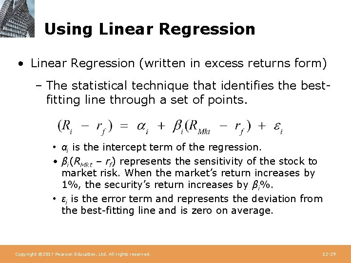
Using Linear Regression • Linear Regression (written in excess returns form) – The statistical technique that identifies the bestfitting line through a set of points. • αi is the intercept term of the regression. • βi(RMkt – rf) represents the sensitivity of the stock to market risk. When the market’s return increases by 1%, the security’s return increases by βi%. • εi is the error term and represents the deviation from the best-fitting line and is zero on average. Copyright © 2017 Pearson Education, Ltd. All rights reserved. 12 -29
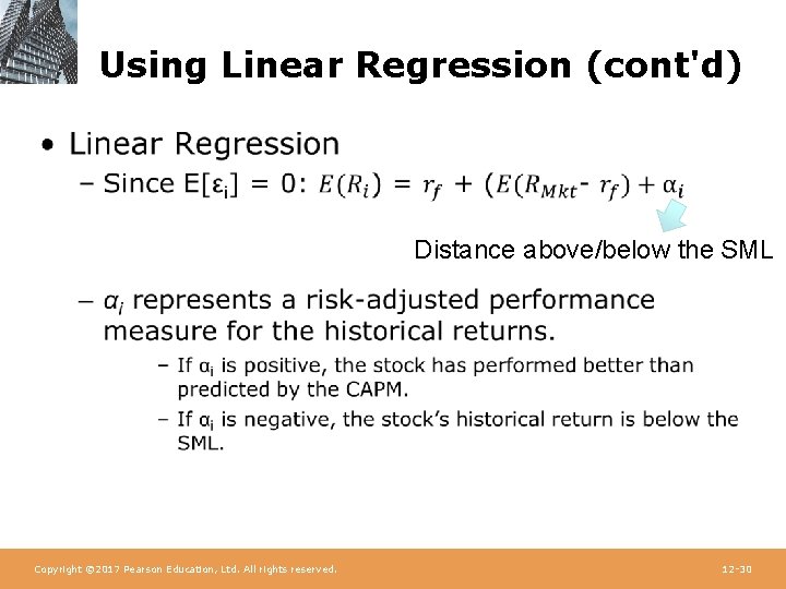
Using Linear Regression (cont'd) • Distance above/below the SML Copyright © 2017 Pearson Education, Ltd. All rights reserved. 12 -30
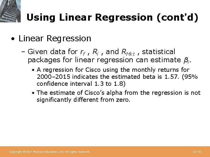
Using Linear Regression (cont'd) • Linear Regression – Given data for rf , Ri , and RMkt , statistical packages for linear regression can estimate βi. • A regression for Cisco using the monthly returns for 2000– 2015 indicates the estimated beta is 1. 57. (95% confidence interval 1. 3 to 1. 8) • The estimate of Cisco’s alpha from the regression is not significantly different from zero. Copyright © 2017 Pearson Education, Ltd. All rights reserved. 12 -31
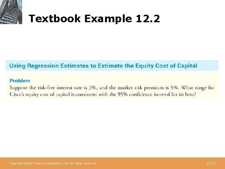
Textbook Example 12. 2 Copyright © 2017 Pearson Education, Ltd. All rights reserved. 12 -32
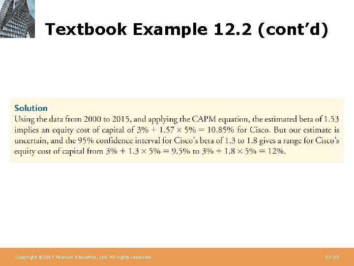
Textbook Example 12. 2 (cont’d) Copyright © 2017 Pearson Education, Ltd. All rights reserved. 12 -33
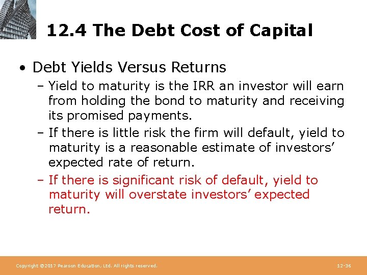
12. 4 The Debt Cost of Capital • Debt Yields Versus Returns – Yield to maturity is the IRR an investor will earn from holding the bond to maturity and receiving its promised payments. – If there is little risk the firm will default, yield to maturity is a reasonable estimate of investors’ expected rate of return. – If there is significant risk of default, yield to maturity will overstate investors’ expected return. Copyright © 2017 Pearson Education, Ltd. All rights reserved. 12 -36
12. 4 The Debt Cost of Capital (cont’d) • Consider a one-year bond with YTM of y. For each $1 invested in the bond today, the issuer promises to pay $(1 + y) in one year. • Suppose the bond will default with probability p, in which case bond holders receive only $(1 + y - L), where L is the expected loss per $1 of debt in the event of default. Copyright © 2017 Pearson Education, Ltd. All rights reserved. 12 -37
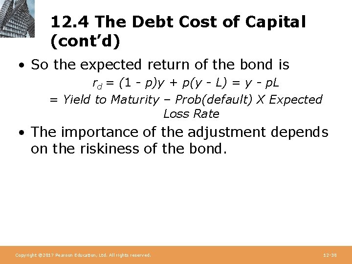
12. 4 The Debt Cost of Capital (cont’d) • So the expected return of the bond is rd = (1 - p)y + p(y - L) = y - p. L = Yield to Maturity – Prob(default) X Expected Loss Rate • The importance of the adjustment depends on the riskiness of the bond. Copyright © 2017 Pearson Education, Ltd. All rights reserved. 12 -38
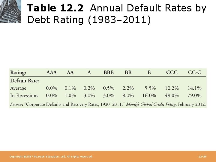
Table 12. 2 Annual Default Rates by Debt Rating (1983– 2011) Copyright © 2017 Pearson Education, Ltd. All rights reserved. 12 -39
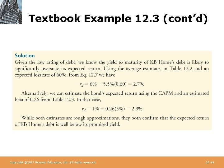
12. 4 The Debt Cost of Capital (cont’d) • The average loss rate for unsecured debt is 60%. • According to Table 12. 2, during average times the annual default rate for B-rated bonds is 5. 5%. • So the expected return to B-rated bondholders during average times is 0. 055 X 0. 60=3. 3% below the bond’s quoted yield. Copyright © 2017 Pearson Education, Ltd. All rights reserved. 12 -40
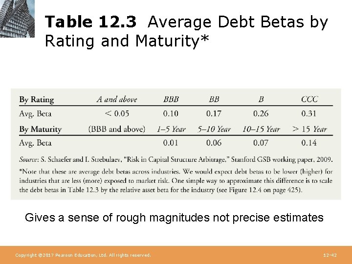
12. 4 The Debt Cost of Capital (cont’d) • Debt Betas – Alternatively, we can estimate the debt cost of capital using the CAPM. – Debt betas are difficult to estimate because corporate bonds are traded infrequently. – One approximation is to use estimates of betas of bond indices by rating category. – Chapter 21 shows an alternative method for estimating debt betas using option prices. Copyright © 2017 Pearson Education, Ltd. All rights reserved. 12 -41
Table 12. 3 Average Debt Betas by Rating and Maturity* Gives a sense of rough magnitudes not precise estimates Copyright © 2017 Pearson Education, Ltd. All rights reserved. 12 -42
Textbook Example 12. 3 Copyright © 2017 Pearson Education, Ltd. All rights reserved. 12 -43
Textbook Example 12. 3 (cont’d) Copyright © 2017 Pearson Education, Ltd. All rights reserved. 12 -44
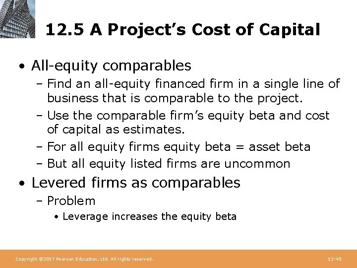
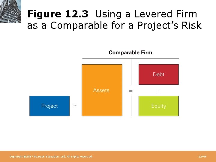
12. 5 A Project’s Cost of Capital • All-equity comparables – Find an all-equity financed firm in a single line of business that is comparable to the project. – Use the comparable firm’s equity beta and cost of capital as estimates. – For all equity firms equity beta = asset beta – But all equity listed firms are uncommon • Levered firms as comparables – Problem • Leverage increases the equity beta Copyright © 2017 Pearson Education, Ltd. All rights reserved. 12 -48
Figure 12. 3 Using a Levered Firm as a Comparable for a Project’s Risk Copyright © 2017 Pearson Education, Ltd. All rights reserved. 12 -49
Textbook Example 12. 4 Copyright © 2017 Pearson Education, Ltd. All rights reserved. 12 -50
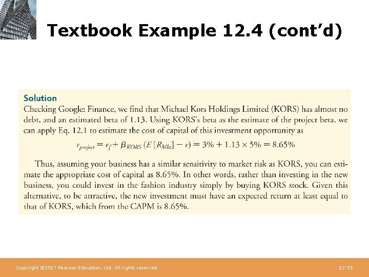
Textbook Example 12. 4 (cont’d) Copyright © 2017 Pearson Education, Ltd. All rights reserved. 12 -51
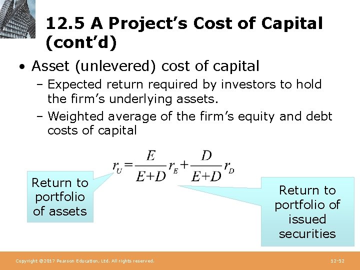
12. 5 A Project’s Cost of Capital (cont’d) • Asset (unlevered) cost of capital – Expected return required by investors to hold the firm’s underlying assets. – Weighted average of the firm’s equity and debt costs of capital Return to portfolio of assets Copyright © 2017 Pearson Education, Ltd. All rights reserved. Return to portfolio of issued securities 12 -52
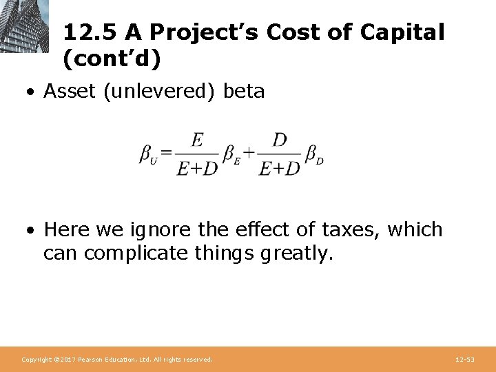
12. 5 A Project’s Cost of Capital (cont’d) • Asset (unlevered) beta • Here we ignore the effect of taxes, which can complicate things greatly. Copyright © 2017 Pearson Education, Ltd. All rights reserved. 12 -53
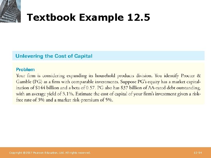
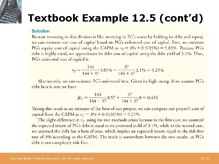
Textbook Example 12. 5 Copyright © 2017 Pearson Education, Ltd. All rights reserved. 12 -54
Textbook Example 12. 5 (cont’d) Copyright © 2017 Pearson Education, Ltd. All rights reserved. 12 -55
Cash and Net Debt • Some firms maintain high cash balances. • Cash is a risk-free asset that reduces the average risk of the firm’s assets. • Because the risk of the firm’s enterprise value (assets - cash = MV issued securities - cash) is what we’re usually concerned with, leverage should be measured in terms of net debt. Net Debt = Debt – Excess Cash and short-term (near cash) investments Copyright © 2017 Pearson Education, Ltd. All rights reserved. 12 -56
Textbook Example 12. 6 Copyright © 2017 Pearson Education, Ltd. All rights reserved. 12 -57
Textbook Example 12. 6 (cont’d) Copyright © 2017 Pearson Education, Ltd. All rights reserved. 12 -58
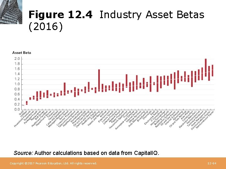
Industry Asset Betas • We can combine estimates of asset betas for multiple firms in the same industry. • Doing this will reduce the estimation error of the estimated beta for the project. Copyright © 2017 Pearson Education, Ltd. All rights reserved. 12 -61
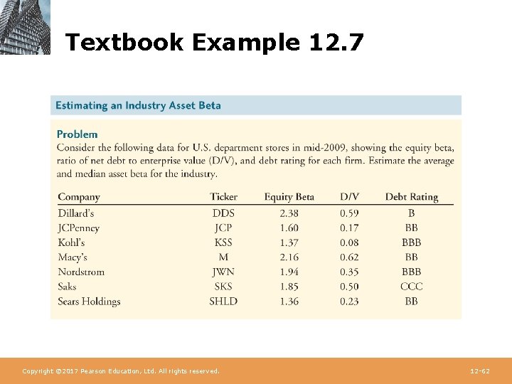
Textbook Example 12. 7 Copyright © 2017 Pearson Education, Ltd. All rights reserved. 12 -62
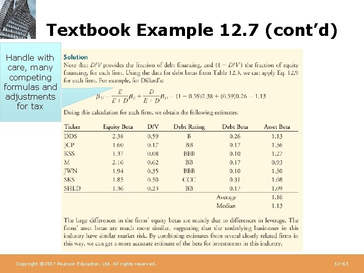
Textbook Example 12. 7 (cont’d) Handle with care, many competing formulas and adjustments for tax Copyright © 2017 Pearson Education, Ltd. All rights reserved. 12 -63
Figure 12. 4 Industry Asset Betas (2016) Source: Author calculations based on data from Capital. IQ. Copyright © 2017 Pearson Education, Ltd. All rights reserved. 12 -64
12. 6 Project Risk Characteristics and Financing • Differences in Project Risk – Firm asset betas reflect market risk of the average project in a firm. – Individual projects may be more or less sensitive to market risk. – In an ideal world each project would have its own discount rate (cost of capital) Copyright © 2017 Pearson Education, Ltd. All rights reserved. 12 -65
12. 6 Project Risk Characteristics and Financing (cont’d) • For example, 3 M has both healthcare and computer display and graphics divisions. • 3 M’s own asset beta represents an average of the risk of these and 3 M’s other divisions. • Financial managers in multidivisional firms should evaluate projects based on asset betas of firms in a similar line of business. – Eg. “Pure play” industry betas Copyright © 2017 Pearson Education, Ltd. All rights reserved. 12 -66
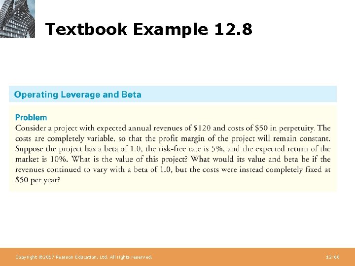
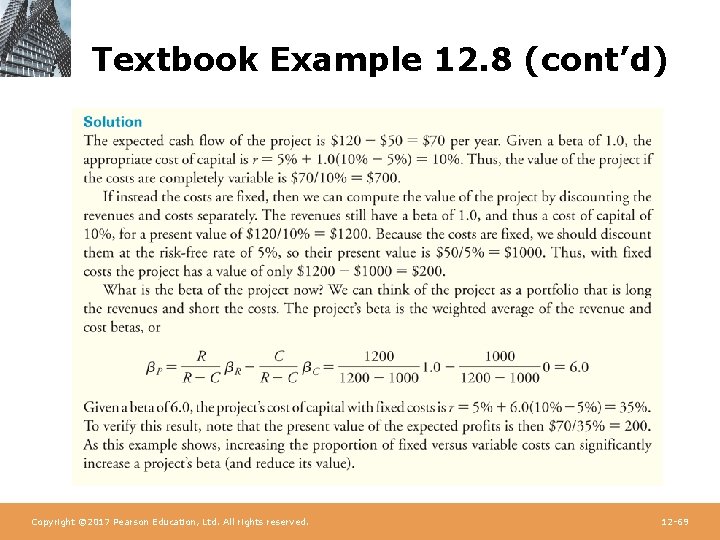
12. 6 Project Risk Characteristics and Financing (cont’d) • Another factor that can affect market risk of a project is its degree of operating leverage. • Operating leverage is the relative proportion of fixed versus variable costs. • A higher proportion of fixed costs increases the sensitivity of the project’s cash flows to market risk. – The project’s beta will be higher. – A higher cost of capital should be assigned. Copyright © 2017 Pearson Education, Ltd. All rights reserved. 12 -67
Textbook Example 12. 8 Copyright © 2017 Pearson Education, Ltd. All rights reserved. 12 -68
Textbook Example 12. 8 (cont’d) Copyright © 2017 Pearson Education, Ltd. All rights reserved. 12 -69
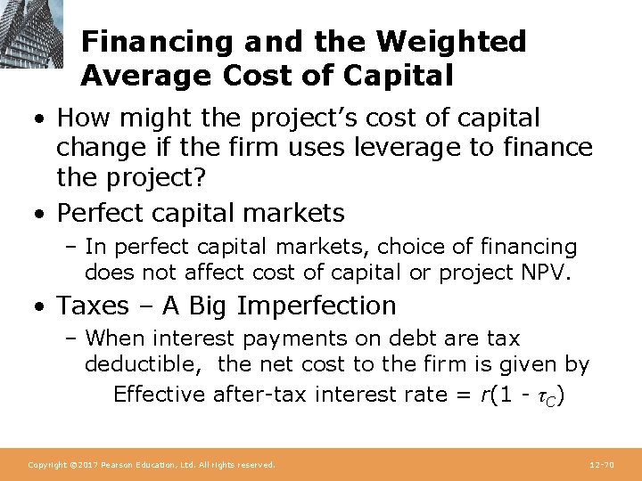
Financing and the Weighted Average Cost of Capital • How might the project’s cost of capital change if the firm uses leverage to finance the project? • Perfect capital markets – In perfect capital markets, choice of financing does not affect cost of capital or project NPV. • Taxes – A Big Imperfection – When interest payments on debt are tax deductible, the net cost to the firm is given by Effective after-tax interest rate = r(1 - τC) Copyright © 2017 Pearson Education, Ltd. All rights reserved. 12 -70
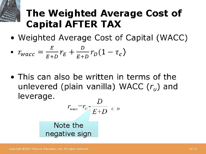
The Weighted Average Cost of Capital AFTER TAX • Note the negative sign Copyright © 2017 Pearson Education, Ltd. All rights reserved. 12 -71
After Tax WACC Under the Imputation Tax System • Copyright © 2017 Pearson Education, Ltd. All rights reserved. 12 -72
The Weighted Average Cost of Capital (cont’d) • How does rwacc compare with r. U? – Unlevered cost of capital (or pretax WACC) • Expected return investors will earn by holding the firm’s assets • In a world with taxes, it can be used to evaluate an allequity project with the same risk as the firm. – In a world with taxes, WACC is less than the expected return of the firm’s assets. • With taxes, WACC can be used to evaluate a project with the same risk and the same financing as the firm. Copyright © 2017 Pearson Education, Ltd. All rights reserved. 12 -73
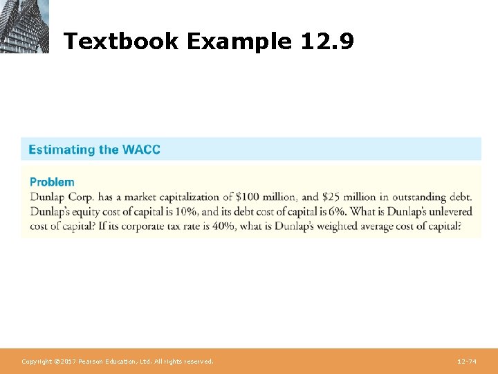
Textbook Example 12. 9 Copyright © 2017 Pearson Education, Ltd. All rights reserved. 12 -74
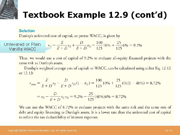
Textbook Example 12. 9 (cont’d) Unlevered or Plain Vanilla WACC Copyright © 2017 Pearson Education, Ltd. All rights reserved. 12 -75
12. 7 Final Thoughts on Using the CAPM • There a large number of assumptions made in the estimation of cost of capital using the CAPM. • How reliable are the results? • Evidence is mixed, but tests generally show the relation between beta and realised (not equilibrium expected) returns seems too flat. – Much debate about what this means, eg: • CAPM doesn’t work OR • Problems with the nature of the tests OR • Investors in low beta stocks are earning “alpha” Copyright © 2017 Pearson Education, Ltd. All rights reserved. 12 -79
Other Asset Pricing Models • Other asset pricing models have been proposed: – After tax CAPM, Black’s zero beta (CAPM) model – Merton’s intertemporal CAPM – Consumption CAPM – Arbitrage Pricing Theory (APT) – Fama and French 3 Factor (now 5 factor)model • Debate over whether this really is an asset pricing model – And…. Several others. • Only the standard CAPM is in common use in estimating the cost of capital for valuation and in capital budgeting. Copyright © 2017 Pearson Education, Ltd. All rights reserved. 12 -80
12. 7 Final Thoughts on Using the CAPM (cont’d) • The types of approximation are no different from those made throughout the capital budgeting process. • CAPM is practical, easy to implement, and robust. • CAPM imposes a disciplined approach to cost of capital estimation that is somewhat difficult to manipulate. • CAPM requires managers to think about risk in the correct way. • Practitioners have chosen the CAPM Copyright © 2017 Pearson Education, Ltd. All rights reserved. 12 -81
Discussion of Data Case Key Topic • In January 2013, Walt Disney Company’s bond rating was A. How would your estimate of the company’s cost of debt change if their bond rating was B or below? Would the yields you observe on the FINRA website be different? Copyright © 2017 Pearson Education, Ltd. All rights reserved. 12 -82
Chapter Quiz 1. What inputs do we need to estimate a firm’s equity cost of capital using the CAPM? 2. How do you determine the weight of a stock in the market portfolio? 3. How can you estimate the market risk premium? 4. How can you estimate a stock’s beta from historical returns? Copyright © 2017 Pearson Education, Ltd. All rights reserved. 12 -83
Chapter Quiz 5. Why does the yield to maturity of a firm’s debt generally overestimate its debt cost of capital? 6. Describe two methods that can be used to estimate a firm’s debt cost of capital. 7. What data can we use to estimate the beta of a project? 8. Why does the equity beta of a levered firm differ from the beta of its assets? Copyright © 2017 Pearson Education, Ltd. All rights reserved. 12 -84
Chapter Quiz 9. Why might projects within the same firm have different costs of capital? 10. Even if the CAPM is not perfect, why might we continue to use it in corporate finance? Copyright © 2017 Pearson Education, Ltd. All rights reserved. 12 -85
Chapter 12 Appendix Copyright © 2017 Pearson Education, Ltd. All rights reserved. 12 -
Practical Considerations When Forecasting Beta 12 A. 1 Time Horizon – For stocks, common practice is to use at least two years of weekly return data or five years of monthly return data. 12 A. 2 The Market Proxy – In practice the S&P 500 is used as the market proxy. Other proxies include the NYSE Composite Index and the Wilshire 5000. Copyright © 2017 Pearson Education, Ltd. All rights reserved. 12 -87
Practical Considerations When Forecasting Beta (cont’d) 12 A. 3 Beta Variation and Extrapolation – Betas vary over time, so many practitioners prefer to use average industry betas rather than individual stock betas. – In addition, evidence suggests that betas tend to regress toward the average beta of 1. 0 over time. Copyright © 2017 Pearson Education, Ltd. All rights reserved. 12 -88
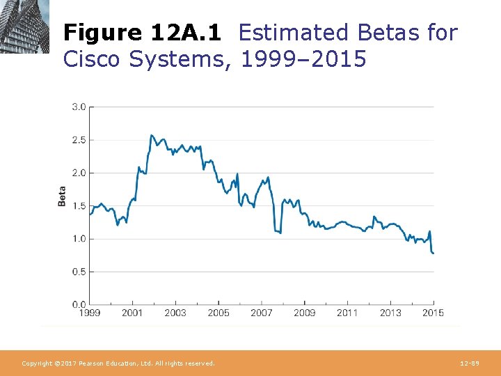
Figure 12 A. 1 Estimated Betas for Cisco Systems, 1999– 2015 Copyright © 2017 Pearson Education, Ltd. All rights reserved. 12 -89
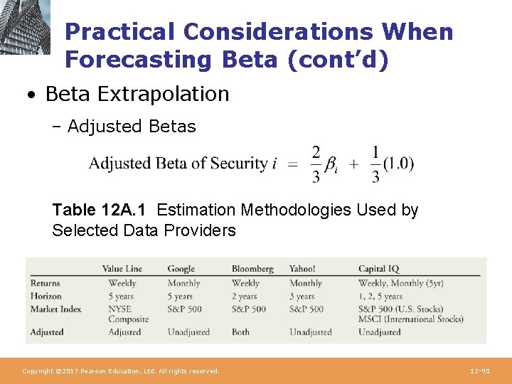
Practical Considerations When Forecasting Beta (cont’d) • Beta Extrapolation – Adjusted Betas Table 12 A. 1 Estimation Methodologies Used by Selected Data Providers Copyright © 2017 Pearson Education, Ltd. All rights reserved. 12 -90
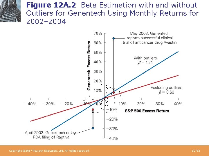
Practical Considerations When Forecasting Beta (cont’d) • 12 A. 4 Outliers – The beta estimates obtained from linear regression can be very sensitive to outliers, which are returns of unusually large magnitude. Copyright © 2017 Pearson Education, Ltd. All rights reserved. 12 -91
Figure 12 A. 2 Beta Estimation with and without Outliers for Genentech Using Monthly Returns for 2002– 2004 Copyright © 2017 Pearson Education, Ltd. All rights reserved. 12 -92
Practical Considerations When Forecasting Beta (cont’d) 12 A. 5 Other Considerations – Changes in the environment of the firm may cause the future to differ from the past. – Many practitioners analyze additional information in addition to past returns. Copyright © 2017 Pearson Education, Ltd. All rights reserved. 12 -93