CONSTRUCTION MANAGEMENT AND ADMINISTRATION UNITV Optimisation UnitV List

CONSTRUCTION MANAGEMENT AND ADMINISTRATION UNIT-V Optimisation

Unit-V: List of topics 1. Introduction 2. Optimisation through linear programming 3. Formulation of LPP 4. Applications of linear programming 5. Graphical method 6. Advantages of LP 7. Limitations of LP 8. Simplex method References: “Operations Research” by SD Sharma “Optimization Methods” D Nagesh Kumar, IISc, Bangalore NPTEL web

Introduction Optimization is the selection of a best element (with regard to some criteria) from some set of available alternatives • Numerical Methods of Optimization – – – – – Linear programming Integer programming Quadratic programming Nonlinear programming Stochastic programming Dynamic programming Combinatorial optimization Infinite-dimensional optimization Constraint satisfaction

Optimisation through linear programming • Linear programming is a technique for determining an optimum schedule of interdependent activities in view of the available resources and constraints • Programming is just another word for planning and refers to the process of determining a particular plan of action from amongst several alternatives • The word linear stands for indicating that all relationships involved in a particular problem are linear • Linear programming indicates the right combination of the various decision variables which can be best employed to achieve the objective taking full account of the practical limitations with in which the problem must be solved • Linear programming problems consist of a linear objective (cost) function (consisting of a certain number of variables) which is to be minimized or maximized subject to a certain number of constraints

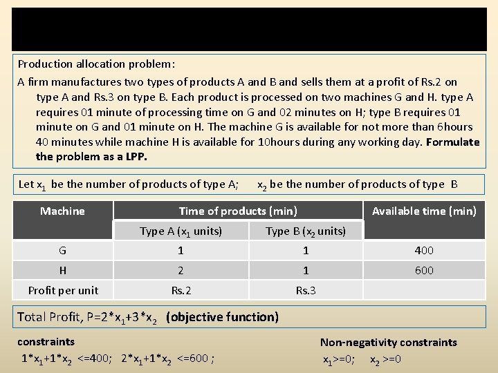
Formulation of LP problems Production allocation problem: A firm manufactures two types of products A and B and sells them at a profit of Rs. 2 on type A and Rs. 3 on type B. Each product is processed on two machines G and H. type A requires 01 minute of processing time on G and 02 minutes on H; type B requires 01 minute on G and 01 minute on H. The machine G is available for not more than 6 hours 40 minutes while machine H is available for 10 hours during any working day. Formulate the problem as a LPP. Let x 1 be the number of products of type A; Machine x 2 be the number of products of type B Time of products (min) Available time (min) Type A (x 1 units) Type B (x 2 units) G 1 1 400 H 2 1 600 Profit per unit Rs. 2 Rs. 3 Total Profit, P=2*x 1+3*x 2 (objective function) constraints 1*x 1+1*x 2 <=400; 2*x 1+1*x 2 <=600 ; Non-negativity constraints x 1>=0; x 2 >=0

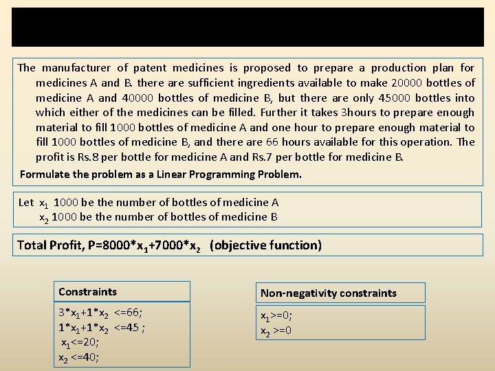
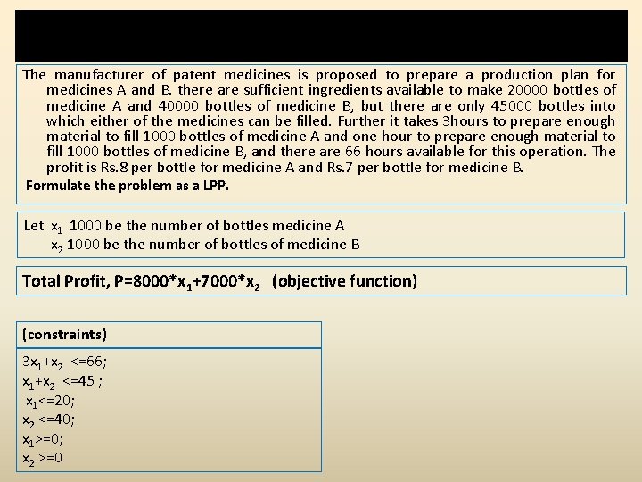
Formulation of LP problems The manufacturer of patent medicines is proposed to prepare a production plan for medicines A and B. there are sufficient ingredients available to make 20000 bottles of medicine A and 40000 bottles of medicine B, but there are only 45000 bottles into which either of the medicines can be filled. Further it takes 3 hours to prepare enough material to fill 1000 bottles of medicine A and one hour to prepare enough material to fill 1000 bottles of medicine B, and there are 66 hours available for this operation. The profit is Rs. 8 per bottle for medicine A and Rs. 7 per bottle for medicine B. Formulate the problem as a Linear Programming Problem. Let x 1 1000 be the number of bottles of medicine A x 2 1000 be the number of bottles of medicine B Total Profit, P=8000*x 1+7000*x 2 (objective function) Constraints Non-negativity constraints 3*x 1+1*x 2 <=66; 1*x 1+1*x 2 <=45 ; x 1<=20; x 2 <=40; x 1>=0; x 2 >=0

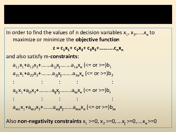
General formulation of LP problem In order to find the values of n decision variables x 1, x 2, . . …xn to maximize or minimize the objective function z = c 1 x 1+ c 2 x 2+ c 3 x 3+……. . cnxn and also satisfy m-constraints: a 11 x 1+a 12 x 2+……. a 1 jxj…. …. a 1 nxn (<= or >=)b 1 a 21 x 1+a 22 x 2+……. . a 2 jxj……. . a 2 nxn (<= or >=)b 2 : : : ai 1 x 1+ai 2 x 2+……. . . aijxj………ainxn (<= or >=)bi : : : am 1 x 1+am 2 x 2+……. amjxj……. amnxn (<= or >=)bm Also non-negativity constraints x 1 >=0, x 2 >=0, …. xj >=0, …. xn >=0

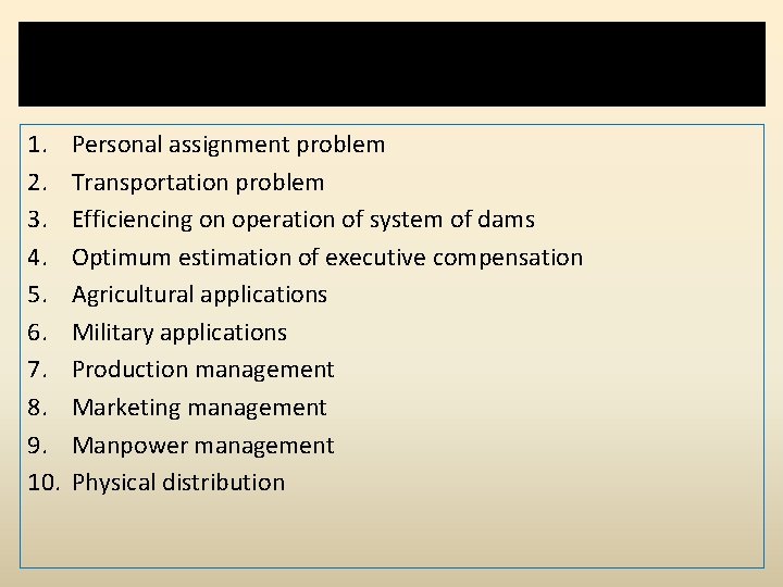
Applications of LP 1. 2. 3. 4. 5. 6. 7. 8. 9. 10. Personal assignment problem Transportation problem Efficiencing on operation of system of dams Optimum estimation of executive compensation Agricultural applications Military applications Production management Marketing management Manpower management Physical distribution

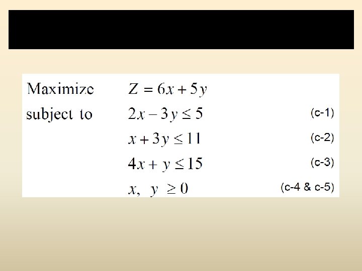
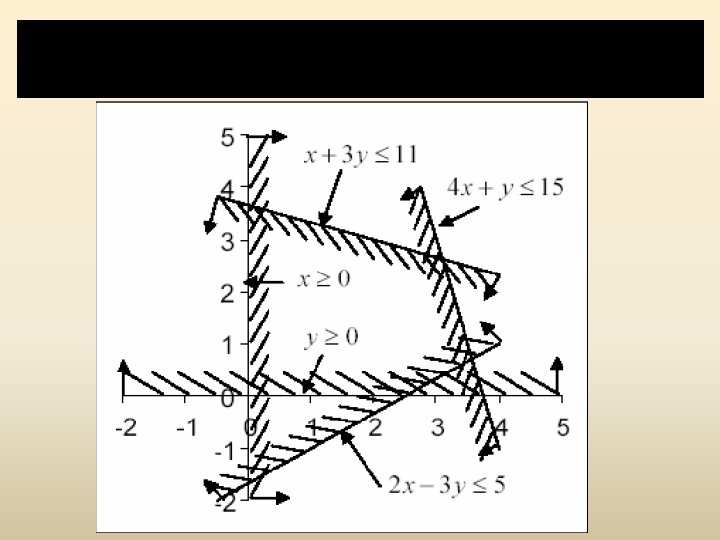
Graphical method (eg. 1)

Step 1: consider each inequality constraint as equation and Plot all the constraints one by one on a graph paper

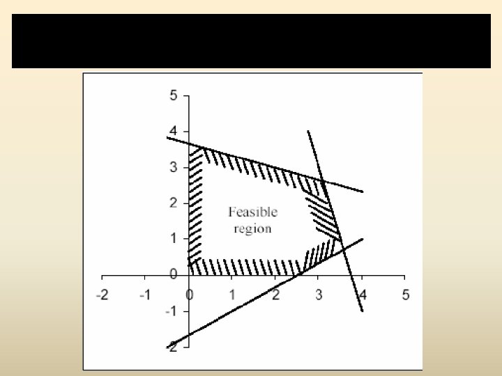
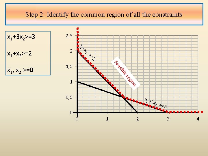
Step 2: Identify the common region of all the constraints

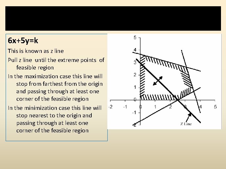
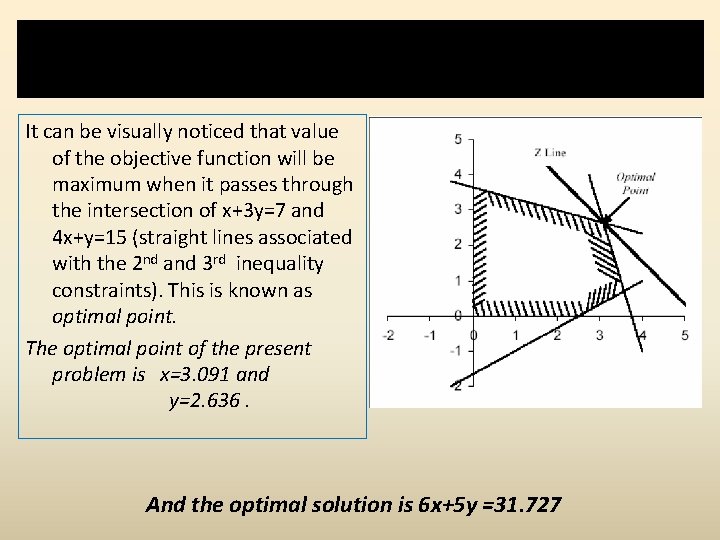
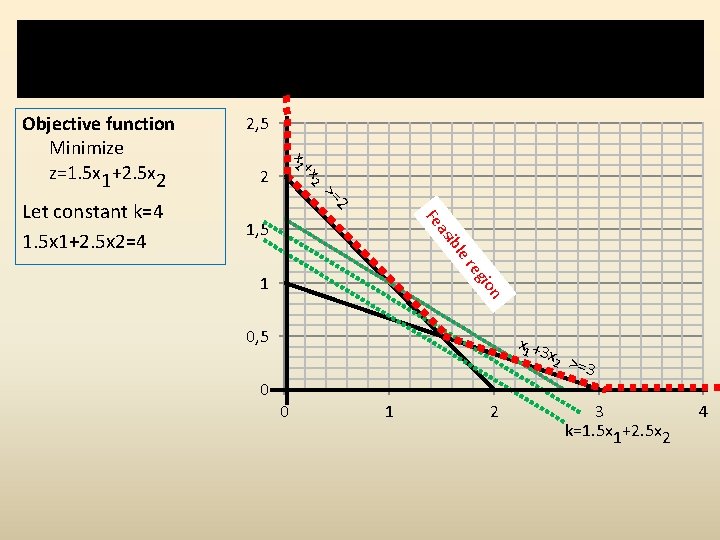
Step 3: Plot the objective function assuming any constant, k 6 x+5 y=k This is known as z line Pull z line until the extreme points of feasible region In the maximization case this line will stop from farthest from the origin and passing through at least one corner of the feasible region In the minimization case this line will stop nearest to the origin and passing through at least one corner of the feasible region

Step 4: Read the coordinates of extreme points and find the maximum/minimum value of z It can be visually noticed that value of the objective function will be maximum when it passes through the intersection of x+3 y=7 and 4 x+y=15 (straight lines associated with the 2 nd and 3 rd inequality constraints). This is known as optimal point. The optimal point of the present problem is x=3. 091 and y=2. 636. And the optimal solution is 6 x+5 y =31. 727

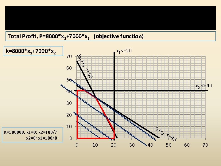
Graphical method (eg. 2) The manufacturer of patent medicines is proposed to prepare a production plan for medicines A and B. there are sufficient ingredients available to make 20000 bottles of medicine A and 40000 bottles of medicine B, but there are only 45000 bottles into which either of the medicines can be filled. Further it takes 3 hours to prepare enough material to fill 1000 bottles of medicine A and one hour to prepare enough material to fill 1000 bottles of medicine B, and there are 66 hours available for this operation. The profit is Rs. 8 per bottle for medicine A and Rs. 7 per bottle for medicine B. Formulate the problem as a LPP. Let x 1 1000 be the number of bottles medicine A x 2 1000 be the number of bottles of medicine B Total Profit, P=8000*x 1+7000*x 2 (objective function) (constraints) 3 x 1+x 2 <=66; x 1+x 2 <=45 ; x 1<=20; x 2 <=40; x 1>=0; x 2 >=0

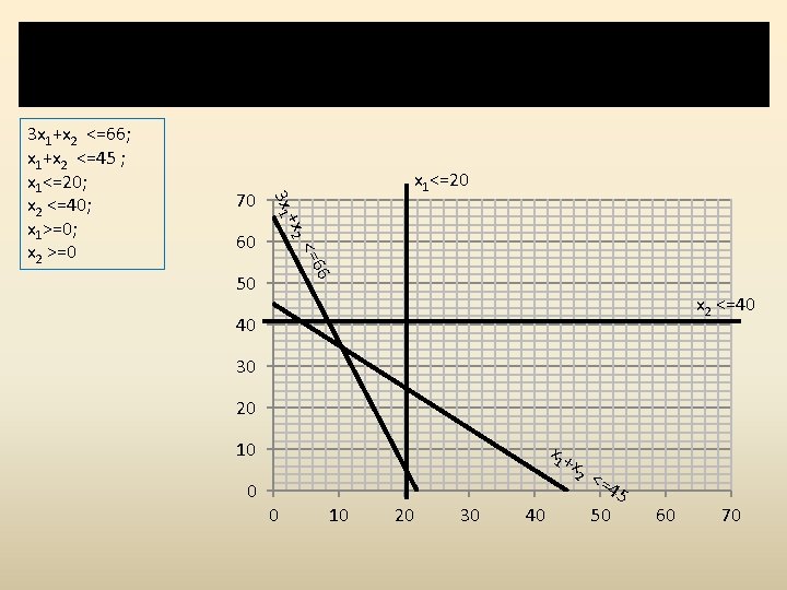
Step 1: consider each inequality constraint as equation and Plot all the constraints one by one on a graph paper 70 6 <=6 60 x 1<=20 +x 2 3 x 1+x 2 <=66; x 1+x 2 <=45 ; x 1<=20; x 2 <=40; x 1>=0; x 2 >=0 50 x 2 <=40 40 30 20 x 1 + 10 0 x 2 0 10 20 30 40 <= 45 50 60 70

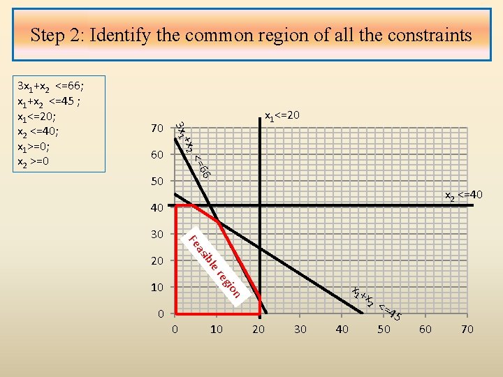
Step 2: Identify the common region of all the constraints 70 6 <=6 60 x 1<=20 +x 2 3 x 1+x 2 <=66; x 1+x 2 <=45 ; x 1<=20; x 2 <=40; x 1>=0; x 2 >=0 50 x 2 <=40 40 as Fe 30 er ibl 20 io eg 0 x 1 + x 2 n 10 0 10 20 30 40 <= 45 50 60 70

Step 3: Plot the objective function assuming any constant, k Total Profit, P=8000*x 1+7000*x 2 (objective function) 70 6 <=6 60 x 1<=20 +x 2 3 x 1 k=8000*x 1+7000*x 2 50 x 2 <=40 40 30 20 K=100000, x 1=0: x 2=100/7 x 2=0; x 1=100/8 x 1 + 10 0 x 2 0 10 20 30 40 <= 45 50 60 70

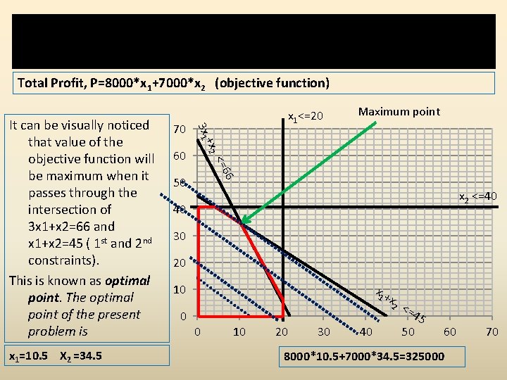
Step 4: Read the coordinates of extreme points and find the maximum/minimum value of z Total Profit, P=8000*x 1+7000*x 2 (objective function) 60 Maximum point <=6 50 6 x 1=10. 5 X 2 =34. 5 70 +x 2 3 x 1 It can be visually noticed that value of the objective function will be maximum when it passes through the intersection of 3 x 1+x 2=66 and x 1+x 2=45 ( 1 st and 2 nd constraints). This is known as optimal point. The optimal point of the present problem is x 1<=20 x 2 <=40 40 30 20 x 1 + 10 0 x 2 0 10 20 30 40 <= 45 50 60 8000*10. 5+7000*34. 5=325000 70

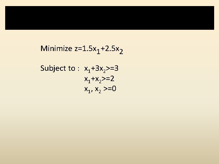
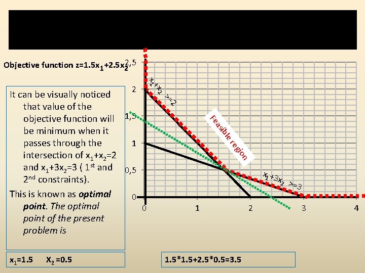
Graphical method (eg. 3) Minimize z=1. 5 x 1+2. 5 x 2 Subject to : x 1+3 x 2>=3 x 1+x 2>=2 x 1, x 2 >=0

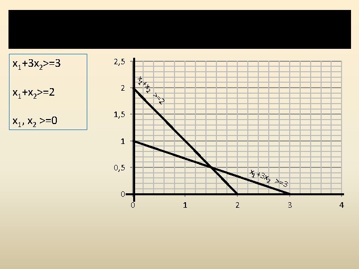
Step 1: consider each inequality constraint as equation and Plot all the constraints one by one on a graph paper x 1+3 x 2>=3 2, 5 x 1, x 2 >=0 1, 5 2 >= 2 +x 2 x 1+x 2>=2 1 0, 5 0 x 1 +3 0 1 2 x 2 > =3 3 4

Step 2: Identify the common region of all the constraints x 1+3 x 2>=3 2, 5 x 1, x 2 >=0 1, 5 2 >= 2 +x 2 x 1+x 2>=2 Fe e ibl as re gio 1 n 0, 5 0 x 1 +3 0 1 2 x 2 > =3 3 4

Step 3: Plot the objective function assuming any constant, k 2 2 >= Fe 1, 5 e ibl as Let constant k=4 1. 5 x 1+2. 5 x 2=4 2, 5 +x 2 x 1 Objective function Minimize z=1. 5 x 1+2. 5 x 2 re gio 1 n 0, 5 0 x 1 +3 x 2 > =3 0 1 2 3 k=1. 5 x 1+2. 5 x 2 4

Step 4: Read the coordinates of extreme points and find the maximum/minimum value of z Objective function z=1. 5 x 1+2. 5 x 22, 5 +x 2 x 1 2 Fe er ibl as ion eg X 2 =0. 5 2 x 1=1. 5 >= It can be visually noticed that value of the objective function will 1, 5 be minimum when it passes through the 1 intersection of x 1+x 2=2 and x 1+3 x 2=3 ( 1 st and 0, 5 2 nd constraints). This is known as optimal 0 point. The optimal 0 point of the present problem is x 1 +3 x 2 > =3 1 1. 5*1. 5+2. 5*0. 5=3. 5 2 3 4

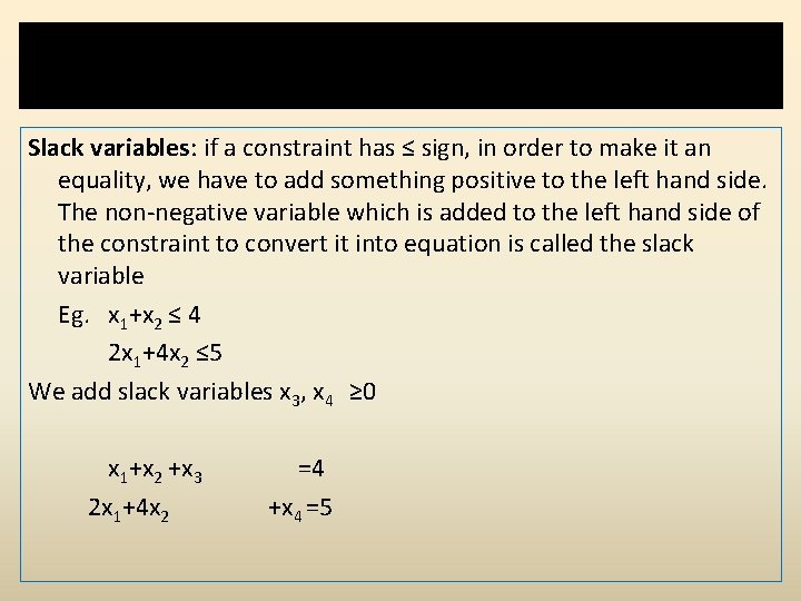
Slack and Surplus variables Slack variables: if a constraint has ≤ sign, in order to make it an equality, we have to add something positive to the left hand side. The non-negative variable which is added to the left hand side of the constraint to convert it into equation is called the slack variable Eg. x 1+x 2 ≤ 4 2 x 1+4 x 2 ≤ 5 We add slack variables x 3, x 4 ≥ 0 x 1+x 2 +x 3 2 x 1+4 x 2 =4 +x 4 =5

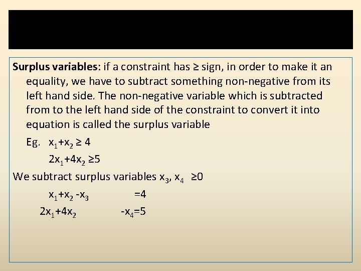
Slack and Surplus variables: if a constraint has ≥ sign, in order to make it an equality, we have to subtract something non-negative from its left hand side. The non-negative variable which is subtracted from to the left hand side of the constraint to convert it into equation is called the surplus variable Eg. x 1+x 2 ≥ 4 2 x 1+4 x 2 ≥ 5 We subtract surplus variables x 3, x 4 ≥ 0 x 1+x 2 -x 3 =4 2 x 1+4 x 2 -x 4=5

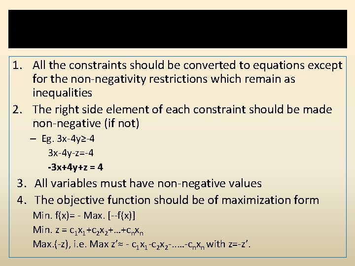
Standard form of LP Problem 1. All the constraints should be converted to equations except for the non-negativity restrictions which remain as inequalities 2. The right side element of each constraint should be made non-negative (if not) – Eg. 3 x-4 y≥-4 3 x-4 y-z=-4 -3 x+4 y+z = 4 3. All variables must have non-negative values 4. The objective function should be of maximization form Min. f(x)= - Max. [--f(x)] Min. z = c 1 x 1+c 2 x 2+…+cnxn Max. (-z), i. e. Max z’≈ - c 1 x 1 -c 2 x 2 -. . …-cnxn with z=-z’.

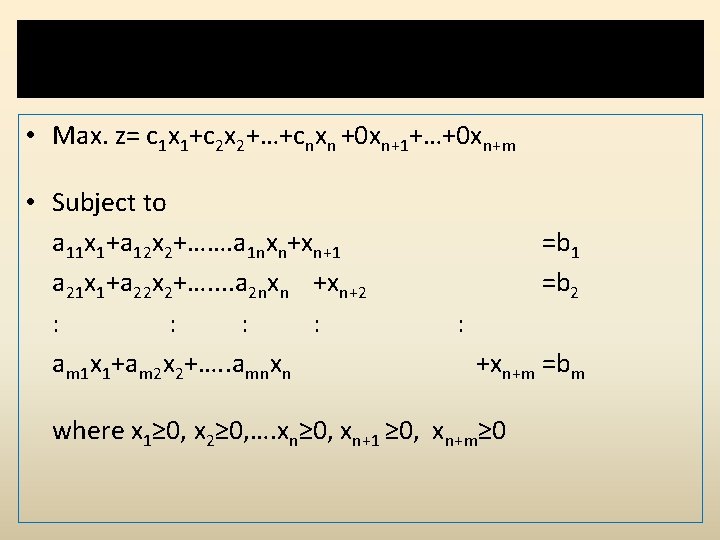
Standard form of general LPP with ≤ constraints • Max. z= c 1 x 1+c 2 x 2+…+cnxn +0 xn+1+…+0 xn+m • Subject to a 11 x 1+a 12 x 2+……. a 1 nxn+xn+1 a 21 x 1+a 22 x 2+…. . a 2 nxn +xn+2 : : am 1 x 1+am 2 x 2+…. . amnxn =b 1 =b 2 : +xn+m =bm where x 1≥ 0, x 2≥ 0, …. xn≥ 0, xn+1 ≥ 0, xn+m≥ 0

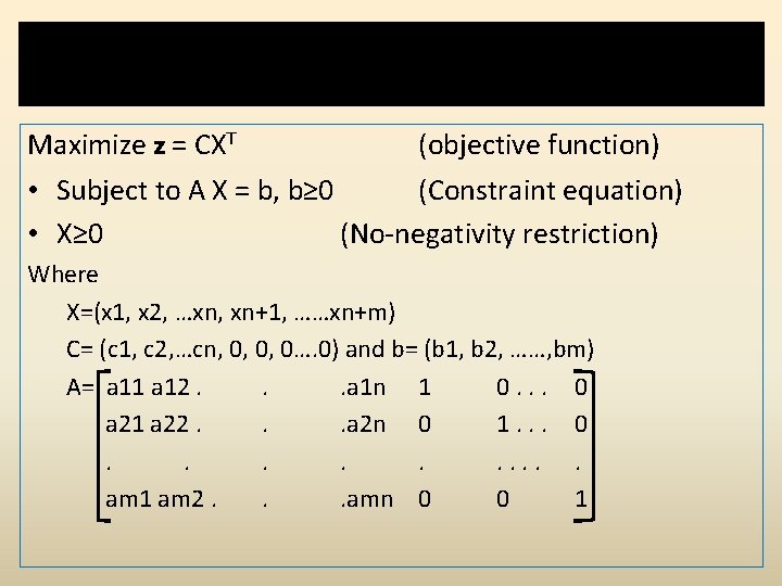
Matrix form of LP Problem Maximize z = CXT (objective function) • Subject to A X = b, b≥ 0 (Constraint equation) • X≥ 0 (No-negativity restriction) Where X=(x 1, x 2, …xn, xn+1, ……xn+m) C= (c 1, c 2, …cn, 0, 0, 0…. 0) and b= (b 1, b 2, ……, bm) A= a 11 a 12. . . a 1 n 1 0. . . 0 a 21 a 22. . . a 2 n 0 1. . . 0. . am 1 am 2. . . amn 0 0 1

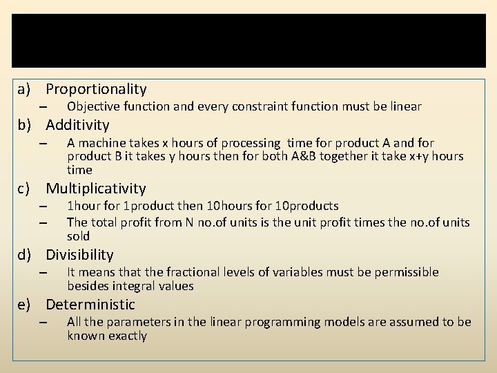
Assumptions in LPP a) Proportionality – Objective function and every constraint function must be linear b) Additivity – A machine takes x hours of processing time for product A and for product B it takes y hours then for both A&B together it take x+y hours time c) Multiplicativity – – 1 hour for 1 product then 10 hours for 10 products The total profit from N no. of units is the unit profit times the no. of units sold d) Divisibility – It means that the fractional levels of variables must be permissible besides integral values e) Deterministic – All the parameters in the linear programming models are assumed to be known exactly

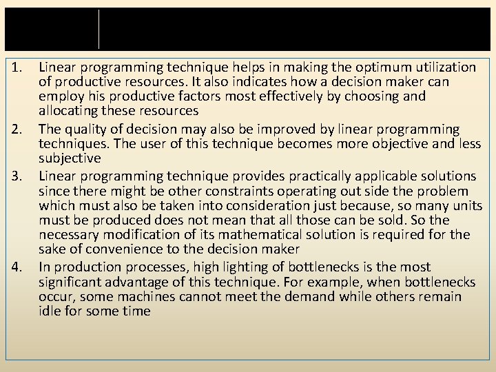
Advantages of LP 1. 2. 3. 4. Linear programming technique helps in making the optimum utilization of productive resources. It also indicates how a decision maker can employ his productive factors most effectively by choosing and allocating these resources The quality of decision may also be improved by linear programming techniques. The user of this technique becomes more objective and less subjective Linear programming technique provides practically applicable solutions since there might be other constraints operating out side the problem which must also be taken into consideration just because, so many units must be produced does not mean that all those can be sold. So the necessary modification of its mathematical solution is required for the sake of convenience to the decision maker In production processes, high lighting of bottlenecks is the most significant advantage of this technique. For example, when bottlenecks occur, some machines cannot meet the demand while others remain idle for some time

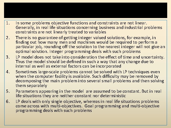
Limitations of LP 1. 2. 3. 4. 5. 6. In some problems objective functions and constraints are not linear. Generally, in real life situations concerning business and industrial problems constraints are not linearly treated to variables There is no guarantee of getting integer valued solutions, for example, in finding out how many men and machines would be required to perform a particular job, rounding off the solution to the nearest integer will not give an optimal solution. Integer programming deals with such problems LP model does not take into consideration the effect of time and uncertainty. Thus the model should be defined in such a way that any change due to internal as well as external factors can be incorporated Sometimes large-scale problems cannot be solved with LP techniques even when the computer facility is available. Such difficulty may be removed by decomposing the main problem into several small problems and then solving them separately Parameters appearing in the model are assumed to be constant. But in real life situations they are neither constant nor deterministic LP deals with only single objective, whereas in real life situations problems come across with multi-objectives. Goal programming and multi-objective programming deals with such problems

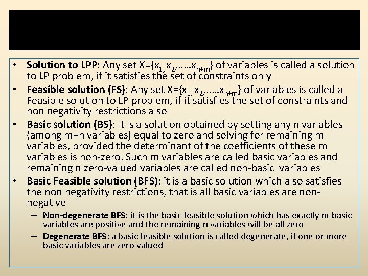
Some Important definitions • Solution to LPP: Any set X={x 1, x 2, . . …xn+m} of variables is called a solution to LP problem, if it satisfies the set of constraints only • Feasible solution (FS): Any set X={x 1, x 2, . . …xn+m} of variables is called a Feasible solution to LP problem, if it satisfies the set of constraints and non negativity restrictions also • Basic solution (BS): it is a solution obtained by setting any n variables (among m+n variables) equal to zero and solving for remaining m variables, provided the determinant of the coefficients of these m variables is non-zero. Such m variables are called basic variables and remaining n zero-valued variables are called non-basic variables • Basic Feasible solution (BFS): it is a basic solution which also satisfies the non negativity restrictions, that is all basic variables are nonnegative – Non-degenerate BFS: it is the basic feasible solution which has exactly m basic variables are positive and the remaining n variables will be all zero – Degenerate BFS: a basic feasible solution is called degenerate, if one or more basic variables are zero valued

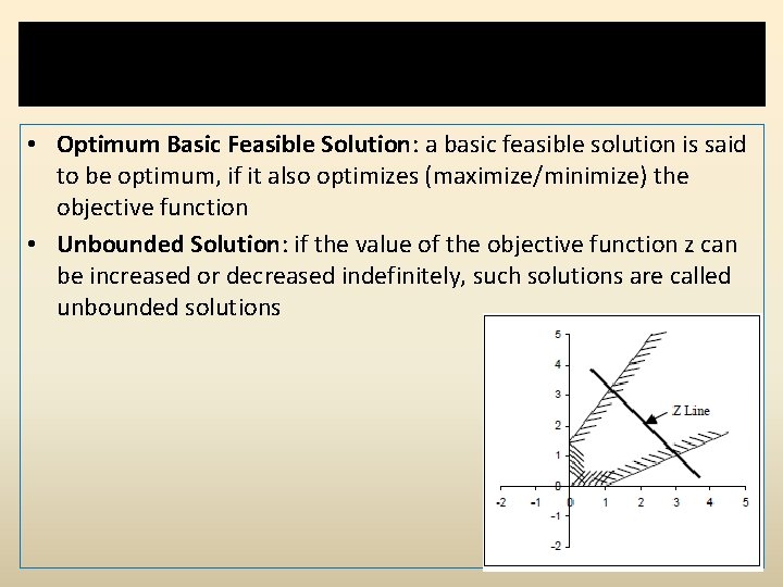
Some Important definitions • Optimum Basic Feasible Solution: a basic feasible solution is said to be optimum, if it also optimizes (maximize/minimize) the objective function • Unbounded Solution: if the value of the objective function z can be increased or decreased indefinitely, such solutions are called unbounded solutions

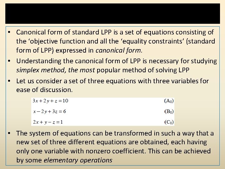
Canonical form of standard LPP • Canonical form of standard LPP is a set of equations consisting of the ‘objective function and all the ‘equality constraints’ (standard form of LPP) expressed in canonical form. • Understanding the canonical form of LPP is necessary for studying simplex method, the most popular method of solving LPP • Let us consider a set of three equations with three variables for ease of discussion. • The system of equations can be transformed in such a way that a new set of three different equations are obtained, each having only one variable with nonzero coefficient. This can be achieved by some elementary operations

Canonical form of standard LPP cont. . . • The following operations are known as elementary operations. – Any equation Er can be replaced by k. Er, where k is a nonzero constant – Any equation Er can be replaced by Er + k. Es, where Es is another equation of the system and k is as defined above • Note that the transformed set of equations through elementary operations is equivalent to the original set of equations. Thus, solution of the transformed set of equations will be the solution of the original set of equations too • Now, let us transform the above set of equations (A 0, B 0 and C 0) through elementary operations

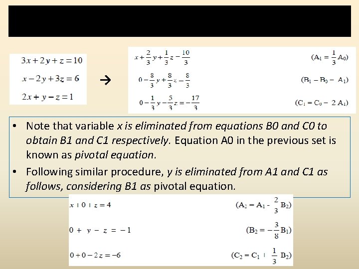
Canonical form of standard LPP cont. . . → • Note that variable x is eliminated from equations B 0 and C 0 to obtain B 1 and C 1 respectively. Equation A 0 in the previous set is known as pivotal equation. • Following similar procedure, y is eliminated from A 1 and C 1 as follows, considering B 1 as pivotal equation.

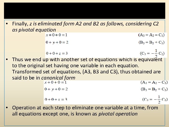
Canonical form of standard LPP cont. . . • Finally, z is eliminated form A 2 and B 2 as follows, considering C 2 as pivotal equation • Thus we end up with another set of equations which is equivalent to the original set having one variable in each equation. Transformed set of equations, (A 3, B 3 and C 3), thus obtained are said to be in canonical form • Operation at each step to eliminate one variable at a time, from all equations except one, is known as pivotal operation

Simplex method • Simplex method is the most popular method used for the solution of Linear Programming Problems (LPP) • Solution of a LPP, if exists, lies at one of the vertices of the feasible region. All the basic solutions can be investigated one-by-one to pick up the optimal solution. • For 10 equations with 15 variables there exists 15 C 10= 3003 basic feasible solutions. Too large number to investigate one-by-one. • This can be overcome by simplex method

General procedure of Simplex method 1. General form of given LPP is transformed to its canonical form 2. Find a basic feasible solution of the LPP (there should exist at least one). 3. Move to an adjacent basic feasible solution which is closest to the optimal solution among all other adjacent vertices. 4. Repeat until optimum solution is achieved. Step three involves ‘Simplex Algorithm’

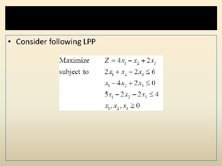
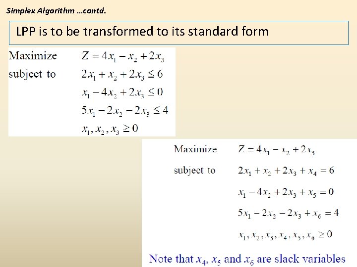
Simplex Algorithm • Consider following LPP

Simplex Algorithm …contd. LPP is to be transformed to its standard form

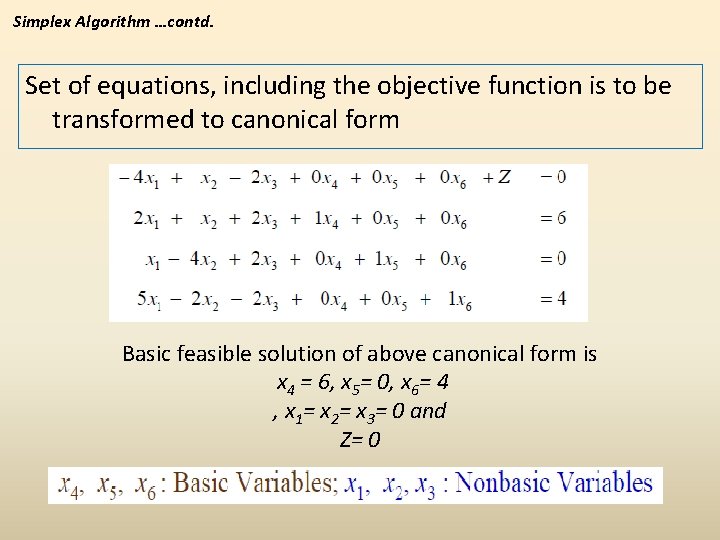
Simplex Algorithm …contd. Set of equations, including the objective function is to be transformed to canonical form Basic feasible solution of above canonical form is x 4 = 6, x 5= 0, x 6= 4 , x 1= x 2= x 3= 0 and Z= 0

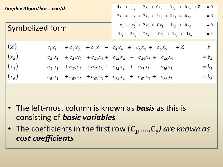
Simplex Algorithm …contd. Symbolized form • The left-most column is known as basis as this is consisting of basic variables • The coefficients in the first row (C 1, . . , C 6) are known as cost coefficients

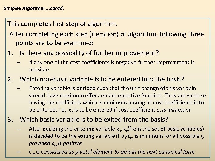
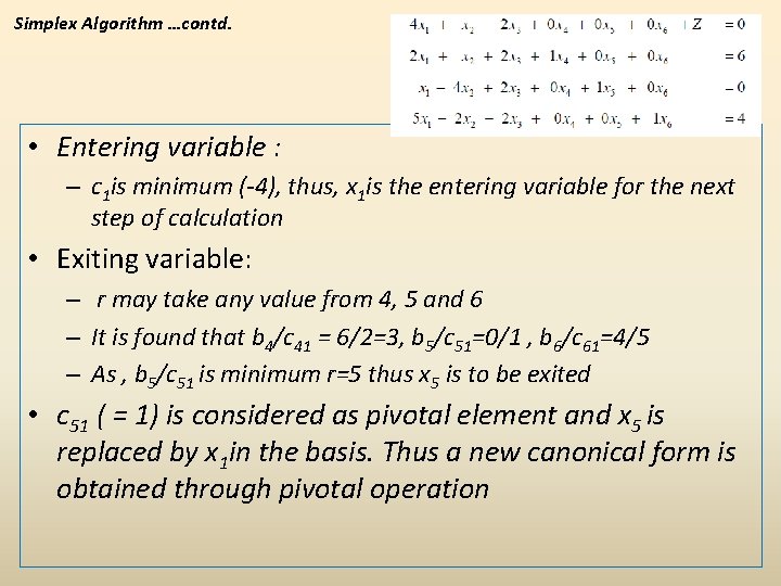
Simplex Algorithm …contd. This completes first step of algorithm. After completing each step (iteration) of algorithm, following three points are to be examined: 1. Is there any possibility of further improvement? – If any one of the cost coefficients is negative further improvement is possible 2. Which non-basic variable is to be entered into the basis? – Entering variable is decided such that the unit change of this variable should have maximum effect on the objective function. Thus the variable having the coefficient which is minimum among all cost coefficients is to be entered, i. e. , xs is to be entered if cost coefficient cs is minimum 3. Which basic variable is to be exited from the basis? – – After deciding the entering variable xs, xr(from the set of basic variables) is decided to be the exiting variable if br/crs is minimum for all possible r, provided crs is positive. Crs is considered as pivotal element to obtain the next canonical form

Simplex Algorithm …contd. • Entering variable : – c 1 is minimum (-4), thus, x 1 is the entering variable for the next step of calculation • Exiting variable: – r may take any value from 4, 5 and 6 – It is found that b 4/c 41 = 6/2=3, b 5/c 51=0/1 , b 6/c 61=4/5 – As , b 5/c 51 is minimum r=5 thus x 5 is to be exited • c 51 ( = 1) is considered as pivotal element and x 5 is replaced by x 1 in the basis. Thus a new canonical form is obtained through pivotal operation

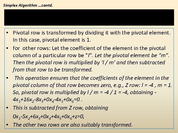
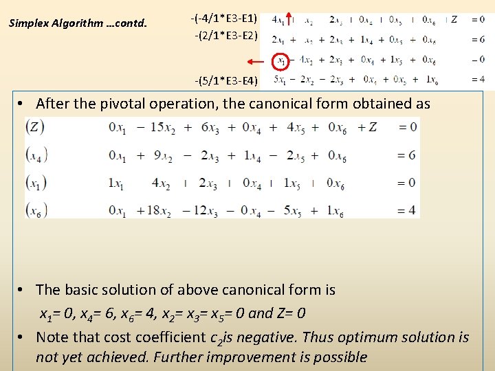
Simplex Algorithm …contd. Pivotal operation • Pivotal row is transformed by dividing it with the pivotal element. In this case, pivotal element is 1. • for other rows: Let the coefficient of the element in the pivotal column of a particular row be “l”. Let the pivotal element be “m”. Then the pivotal row is multiplied by ‘l / m’ and then subtracted from that row to be transformed. • This operation ensures that the coefficients of the element in the pivotal column of that row becomes zero, e. g. , Z row: l = -4 , m = 1. So, pivotal row is multiplied by l / m = -4 / 1 = -4, obtaining 4 x 1+16 x 2 -8 x 3+0 x 4 -4 x 5+0 x 6=0. • This is subtracted from Z row, obtaining 0 x 1 -5 x 2+6 x 3+0 x 4+4 x 5+0 x 6+z=0, • The other two rows are also suitably transformed.

Simplex Algorithm …contd. -(-4/1*E 3 -E 1) -(2/1*E 3 -E 2) -(5/1*E 3 -E 4) • After the pivotal operation, the canonical form obtained as follows • The basic solution of above canonical form is x 1= 0, x 4= 6, x 6= 4, x 2= x 3= x 5= 0 and Z= 0 • Note that cost coefficient c 2 is negative. Thus optimum solution is not yet achieved. Further improvement is possible

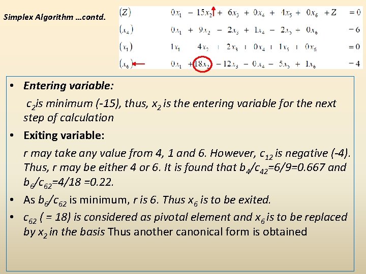
Simplex Algorithm …contd. • Entering variable: c 2 is minimum (-15), thus, x 2 is the entering variable for the next step of calculation • Exiting variable: r may take any value from 4, 1 and 6. However, c 12 is negative (-4). Thus, r may be either 4 or 6. It is found that b 4/c 42=6/9=0. 667 and b 6/c 62=4/18 =0. 22. • As b 6/c 62 is minimum, r is 6. Thus x 6 is to be exited. • c 62 ( = 18) is considered as pivotal element and x 6 is to be replaced by x 2 in the basis Thus another canonical form is obtained

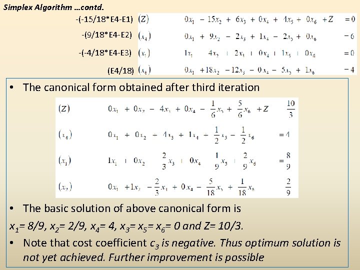
Simplex Algorithm …contd. -(-15/18*E 4 -E 1) -(9/18*E 4 -E 2) -(-4/18*E 4 -E 3) (E 4/18) • The canonical form obtained after third iteration • The basic solution of above canonical form is x 1= 8/9, x 2= 2/9, x 4= 4, x 3= x 5= x 6= 0 and Z= 10/3. • Note that cost coefficient c 3 is negative. Thus optimum solution is not yet achieved. Further improvement is possible

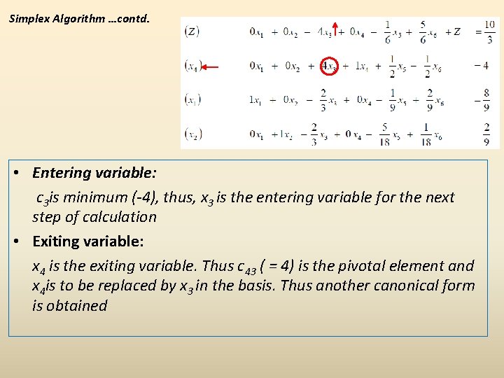
Simplex Algorithm …contd. • Entering variable: c 3 is minimum (-4), thus, x 3 is the entering variable for the next step of calculation • Exiting variable: x 4 is the exiting variable. Thus c 43 ( = 4) is the pivotal element and x 4 is to be replaced by x 3 in the basis. Thus another canonical form is obtained

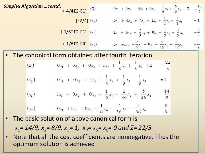
Simplex Algorithm …contd. -(-4/4 E 2 -E 1) (E 2/4) -(-1/6*E 2 -E 3) -(-1/6 E 2 -E 4) • The canonical form obtained after fourth iteration • The basic solution of above canonical form is x 1= 14/9, x 2= 8/9, x 3= 1, x 4= x 5= x 6= 0 and Z= 22/3 • Note that all the cost coefficients are nonnegative. Thus the optimum solution is achieved

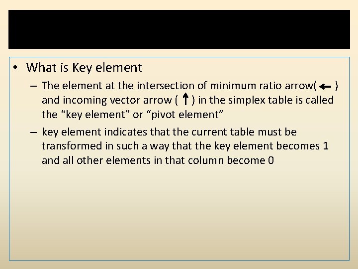
The “key element” or “pivot element” • What is Key element – The element at the intersection of minimum ratio arrow( ) and incoming vector arrow ( ) in the simplex table is called the “key element” or “pivot element” – key element indicates that the current table must be transformed in such a way that the key element becomes 1 and all other elements in that column become 0

Need of artificial variable in LP model • LP problems, in which constraints may also have ≥ and = signs after ensuring that all bi are ≥ 0, are considered in two phase method. In such problems, basis matrix is not obtained as an identity matrix in the starting simplex table, therefore we introduce a new type of variable called the Artificial variable • These variables are fictitious and cannot have any physical meaning • The artificial variable technique is merely a device to get the starting basic feasible solution, so that simplex procedure may be adopted as usual until the optimal solution is obtained • Artificial variables can be eliminated from the simplex table as and they become zero (non-basic)

linear programming in Construction Management Linear programming can be used in construction management to solve many problems such as: 1. Optimizing use of resources 2. Determining most economic product mix. 3. Transportation and routing problems. 4. Personnel assignment. 5. Determining Optimum size of bid. 6. Location of new production plants, offices and warehouses

Examples of use of linear programming in construction A pre-mixed concrete firm has to supply concrete to three different projects A, B, and C. The projects require 200, 350, and 400 cubic meters of concrete in a particular week. The firm has three plants P 1, P 2, and P 3 which can produce 250, 400 and 350 respectively. The cost is different from each Pant to each project since distance will vary. It is required to determine the quantity to be supplied from each plant to each project such that cost to be incurred is a minimum

Assignment -5 • • Applications of LP in construction management Advantages of LP Limitations of LP What is Canonical Form of LP?