Conditional Random Fields and Its Applications Presenter ShihHsiang

Conditional Random Fields and Its Applications Presenter: Shih-Hsiang Lin 06/25/2007

Introduction • The task of assigning label sequences to a set of observation sequences arises in many field – Bioinformatics, Computational linguistics, Speech recognition, Information extraction etc. • One of the most common methods for performing such labeling and segmentation tasks is that of employing hidden Markov models (HMM) or probability finite-state automata – Identify the most likely sequence of labels in any given observation sequences 2

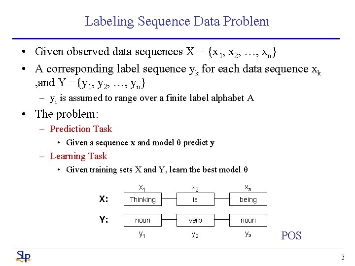
Labeling Sequence Data Problem • Given observed data sequences X = {x 1, x 2, …, xn} • A corresponding label sequence yk for each data sequence xk , and Y ={y 1, y 2, …, yn} – yi is assumed to range over a finite label alphabet A • The problem: – Prediction Task • Given a sequence x and model θ predict y – Learning Task • Given training sets X and Y, learn the best model θ x 1 x 2 x 3 X: Thinking is being Y: noun verb noun y 1 y 2 y 3 POS 3

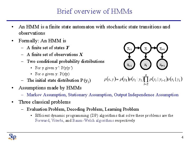
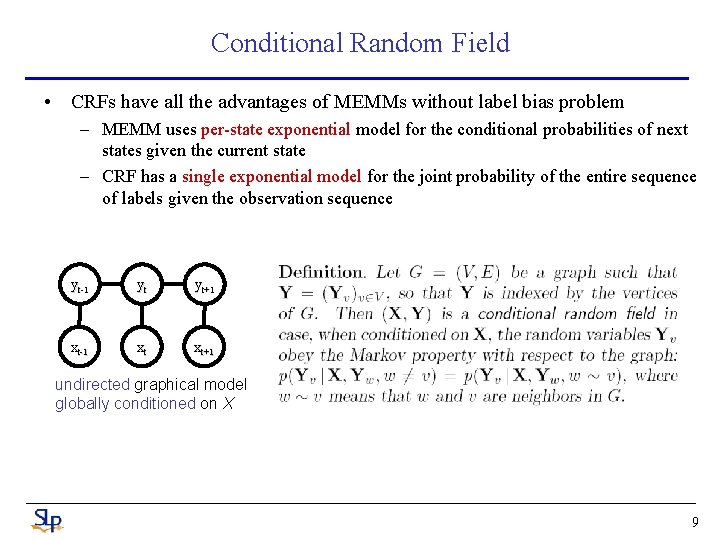
Brief overview of HMMs • An HMM is a finite state automaton with stochastic state transitions and observations • Formally: An HMM is – A finite set of states Y – A finite set of observations X – Two conditional probability distributions • For y given y’: P(y|y’) • For o given y: P(x|y) yt-1 yt yt+1 xt-1 xt xt+1 – The initial state distribution P (y 1) • Assumptions made by HMMs – Markov Assumption, Stationary Assumption, Output Independence Assumption • Three classical problems – Evaluation Problem, Decoding Problem, Learning Problem • Efficient dynamic programming (DP) algorithms that solve these problems are the Forward, Viterbi, and Baum-Welch algorithms respectively 4

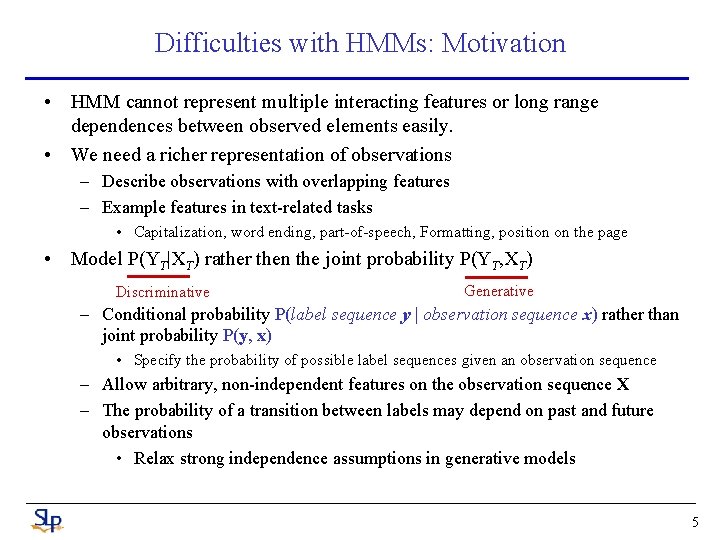
Difficulties with HMMs: Motivation • HMM cannot represent multiple interacting features or long range dependences between observed elements easily. • We need a richer representation of observations – Describe observations with overlapping features – Example features in text-related tasks • Capitalization, word ending, part-of-speech, Formatting, position on the page • Model P(YT|XT) rather then the joint probability P(YT, XT) Discriminative Generative – Conditional probability P(label sequence y | observation sequence x) rather than joint probability P(y, x) • Specify the probability of possible label sequences given an observation sequence – Allow arbitrary, non-independent features on the observation sequence X – The probability of a transition between labels may depend on past and future observations • Relax strong independence assumptions in generative models 5

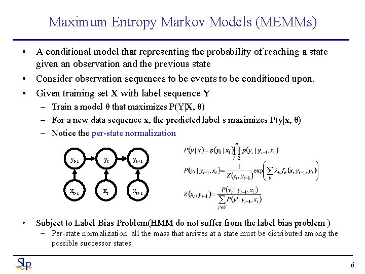
Maximum Entropy Markov Models (MEMMs) • A conditional model that representing the probability of reaching a state given an observation and the previous state • Consider observation sequences to be events to be conditioned upon. • Given training set X with label sequence Y – Train a model θ that maximizes P(Y|X, θ) – For a new data sequence x, the predicted label s maximizes P(y|x, θ) – Notice the per-state normalization • yt-1 yt yt+1 xt-1 xt xt+1 Subject to Label Bias Problem(HMM do not suffer from the label bias problem ) – Per-state normalization: all the mass that arrives at a state must be distributed among the possible successor states 6

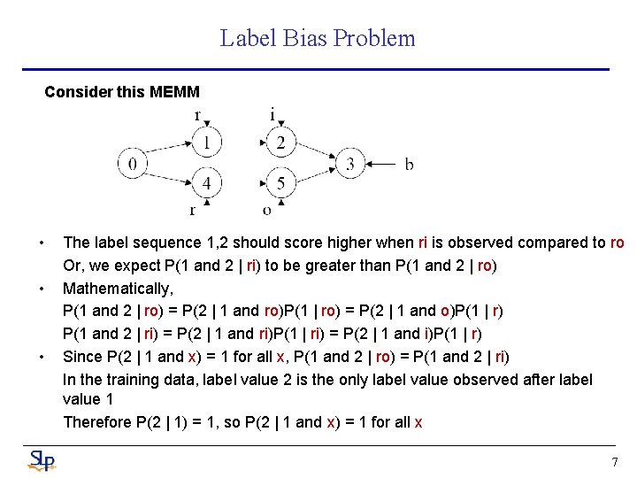
Label Bias Problem Consider this MEMM • • • The label sequence 1, 2 should score higher when ri is observed compared to ro Or, we expect P(1 and 2 | ri) to be greater than P(1 and 2 | ro) Mathematically, P(1 and 2 | ro) = P(2 | 1 and ro)P(1 | ro) = P(2 | 1 and o)P(1 | r) P(1 and 2 | ri) = P(2 | 1 and ri)P(1 | ri) = P(2 | 1 and i)P(1 | r) Since P(2 | 1 and x) = 1 for all x, P(1 and 2 | ro) = P(1 and 2 | ri) In the training data, label value 2 is the only label value observed after label value 1 Therefore P(2 | 1) = 1, so P(2 | 1 and x) = 1 for all x 7

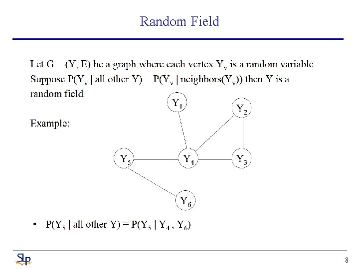
Random Field 8

Conditional Random Field • CRFs have all the advantages of MEMMs without label bias problem – MEMM uses per-state exponential model for the conditional probabilities of next states given the current state – CRF has a single exponential model for the joint probability of the entire sequence of labels given the observation sequence yt-1 yt yt+1 xt-1 xt xt+1 undirected graphical model globally conditioned on X 9

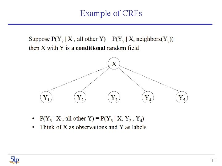
Example of CRFs 10

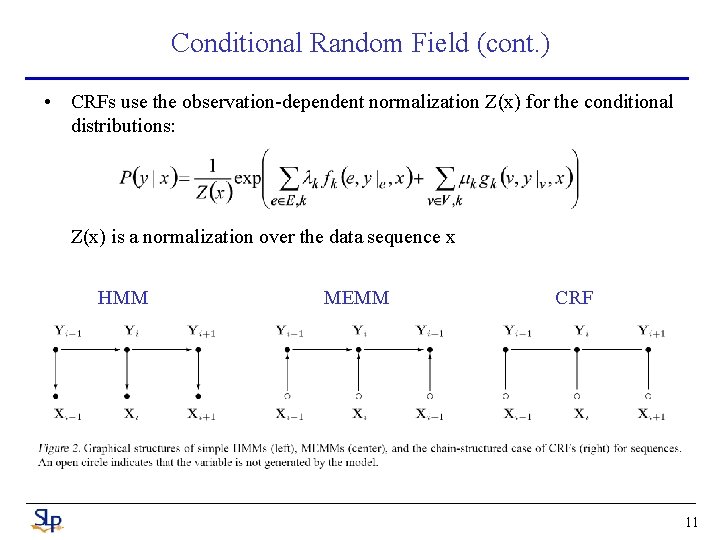
Conditional Random Field (cont. ) • CRFs use the observation-dependent normalization Z(x) for the conditional distributions: Z(x) is a normalization over the data sequence x HMM MEMM CRF 11

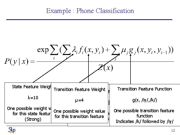
Example : Phone Classification State Feature Weight Transition Feature Function Transition Feature Weight State Feature Function λ=10 g(x, /iy/, /k/) μ=4 f([x is stop], /t/) One possible weight value One possible transition feature One possible weight state value feature One possible function for this state feature function for this transition For our feature attributes and labels (Strong) Indicates /k/ followed by /iy/ 12

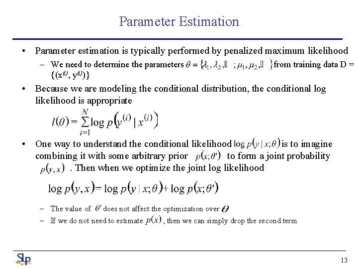
Parameter Estimation • Parameter estimation is typically performed by penalized maximum likelihood – We need to determine the parameters {(x(i), y(i))} from training data D = • Because we are modeling the conditional distribution, the conditional log likelihood is appropriate • One way to understand the conditional likelihood is to imagine combining it with some arbitrary prior to form a joint probability. Then we optimize the joint log likelihood – The value of does not affect the optimization over – If we do not need to estimate , then we can simply drop the second term 13

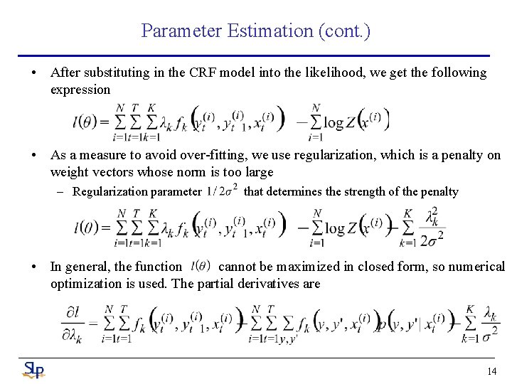
Parameter Estimation (cont. ) • After substituting in the CRF model into the likelihood, we get the following expression • As a measure to avoid over-fitting, we use regularization, which is a penalty on weight vectors whose norm is too large – Regularization parameter that determines the strength of the penalty • In general, the function cannot be maximized in closed form, so numerical optimization is used. The partial derivatives are 14

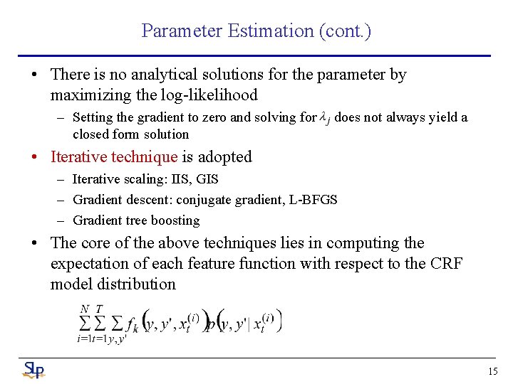
Parameter Estimation (cont. ) • There is no analytical solutions for the parameter by maximizing the log-likelihood – Setting the gradient to zero and solving for closed form solution does not always yield a • Iterative technique is adopted – Iterative scaling: IIS, GIS – Gradient descent: conjugate gradient, L-BFGS – Gradient tree boosting • The core of the above techniques lies in computing the expectation of each feature function with respect to the CRF model distribution 15

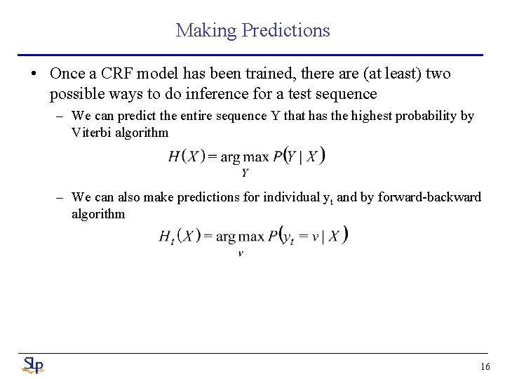
Making Predictions • Once a CRF model has been trained, there are (at least) two possible ways to do inference for a test sequence – We can predict the entire sequence Y that has the highest probability by Viterbi algorithm – We can also make predictions for individual yt and by forward-backward algorithm 16

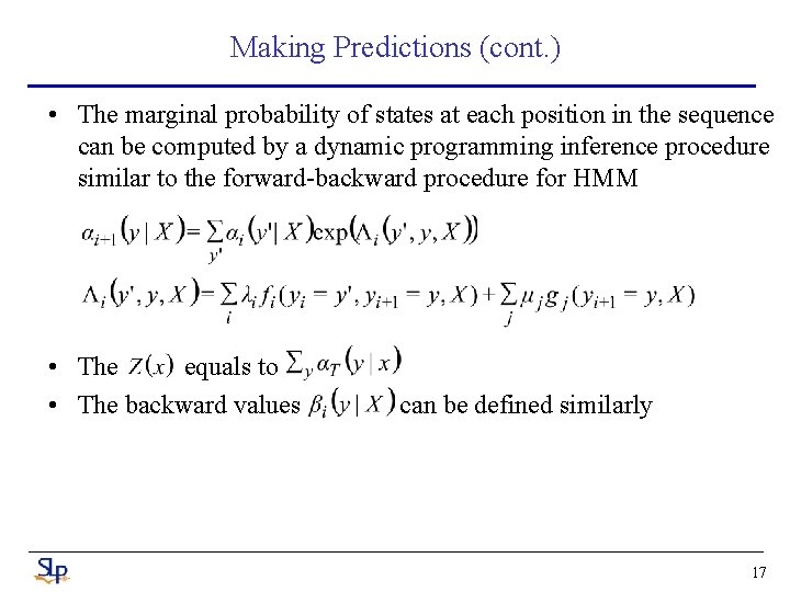
Making Predictions (cont. ) • The marginal probability of states at each position in the sequence can be computed by a dynamic programming inference procedure similar to the forward-backward procedure for HMM • The equals to • The backward values can be defined similarly 17

CRF in Summarization

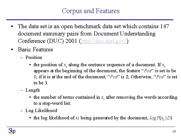
Corpus and Features • The data set is an open benchmark data set which contains 147 document summary pairs from Document Understanding Conference (DUC) 2001 (http: //duc. nist. gov/) • Basic Features – Position • the position of xi along the sentence sequence of a document. If xi appears at the beginning of the document, the feature “Pos” is set to be 1; if it is at the end of the document, “Pos” is 2; Otherwise, “Pos” is set to be 3. – Length • the number of terms contained in xi after removing the words according to a stop-word list. – Log Likelihood • the log likelihood of xi being generated by the document, log. P(xi |D) 19

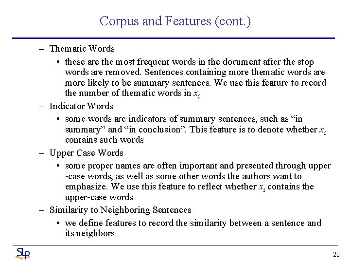
Corpus and Features (cont. ) – Thematic Words • these are the most frequent words in the document after the stop words are removed. Sentences containing more thematic words are more likely to be summary sentences. We use this feature to record the number of thematic words in xi – Indicator Words • some words are indicators of summary sentences, such as “in summary” and “in conclusion”. This feature is to denote whether xi contains such words – Upper Case Words • some proper names are often important and presented through upper -case words, as well as some other words the authors want to emphasize. We use this feature to reflect whether xi contains the upper-case words – Similarity to Neighboring Sentences • we define features to record the similarity between a sentence and its neighbors 20

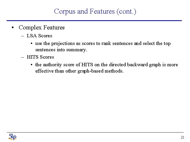
Corpus and Features (cont. ) • Complex Features – LSA Scores • use the projections as scores to rank sentences and select the top sentences into summary. – HITS Scores • the authority score of HITS on the directed backward graph is more effective than other graph-based methods. 21

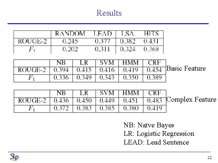
Results Basic Feature Complex Feature NB: Naïve Bayes LR: Logistic Regression LEAD: Lead Sentence 22