Computer Vision Multiple View Geometry Marc Pollefeys COMP

Computer Vision Multiple View Geometry Marc Pollefeys COMP 256

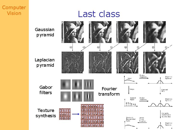
Computer Vision Last class Gaussian pyramid Laplacian pyramid Gabor filters Texture synthesis Fourier transform

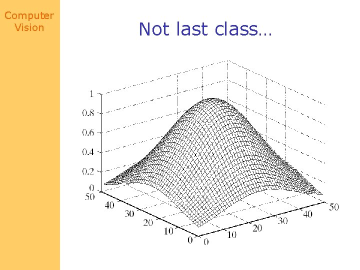
Computer Vision Not last class…

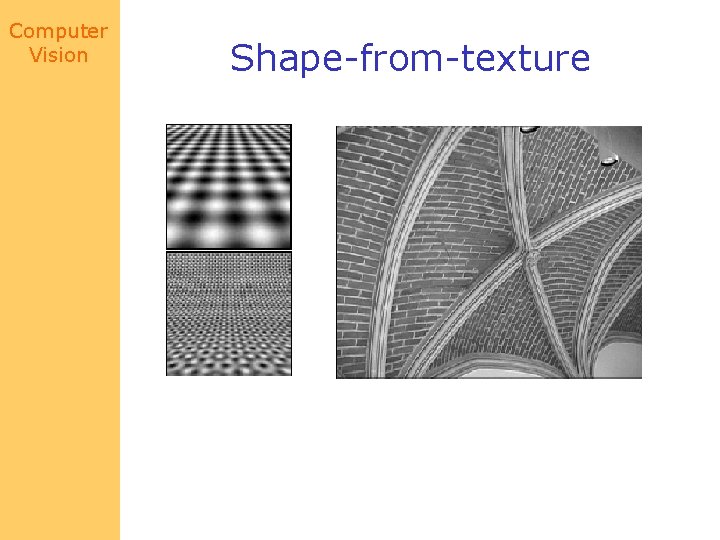
Computer Vision Shape-from-texture

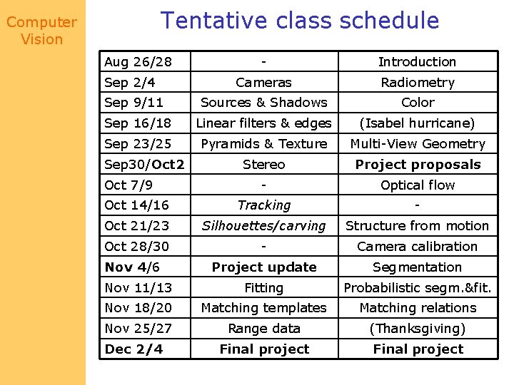
Tentative class schedule Computer Vision Aug 26/28 - Introduction Cameras Radiometry Sources & Shadows Color Sep 16/18 Linear filters & edges (Isabel hurricane) Sep 23/25 Pyramids & Texture Multi-View Geometry Stereo Project proposals - Optical flow Oct 14/16 Tracking - Oct 21/23 Silhouettes/carving Structure from motion Oct 28/30 - Camera calibration Project update Segmentation Nov 11/13 Fitting Probabilistic segm. &fit. Nov 18/20 Matching templates Matching relations Nov 25/27 Range data (Thanksgiving) Final project Sep 2/4 Sep 9/11 Sep 30/Oct 2 Oct 7/9 Nov 4/6 Dec 2/4

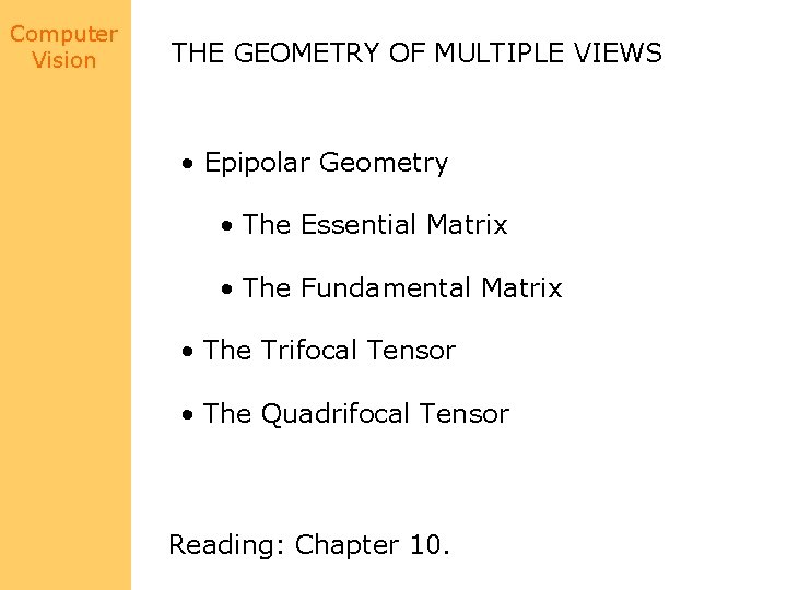
Computer Vision THE GEOMETRY OF MULTIPLE VIEWS • Epipolar Geometry • The Essential Matrix • The Fundamental Matrix • The Trifocal Tensor • The Quadrifocal Tensor Reading: Chapter 10.

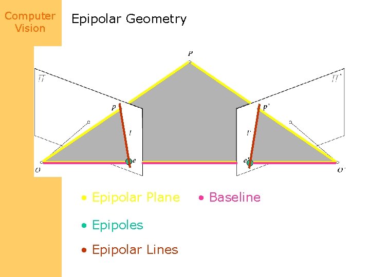
Computer Vision Epipolar Geometry • Epipolar Plane • Epipoles • Epipolar Lines • Baseline

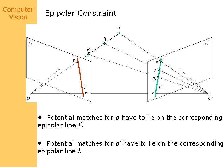
Computer Vision Epipolar Constraint • Potential matches for p have to lie on the corresponding epipolar line l’. • Potential matches for p’ have to lie on the corresponding epipolar line l.

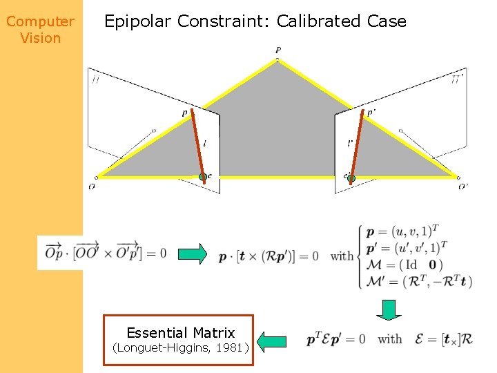
Computer Vision Epipolar Constraint: Calibrated Case Essential Matrix (Longuet-Higgins, 1981)

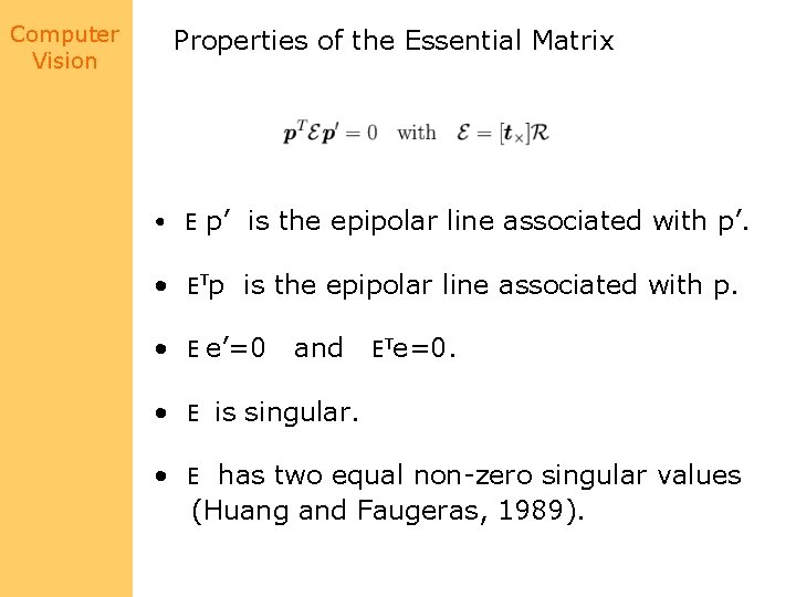
Computer Vision Properties of the Essential Matrix T • E p’ is the epipolar line associated with p’. T • ETp is the epipolar line associated with p. • E e’=0 and ETe=0. • E is singular. • E has two equal non-zero singular values (Huang and Faugeras, 1989).

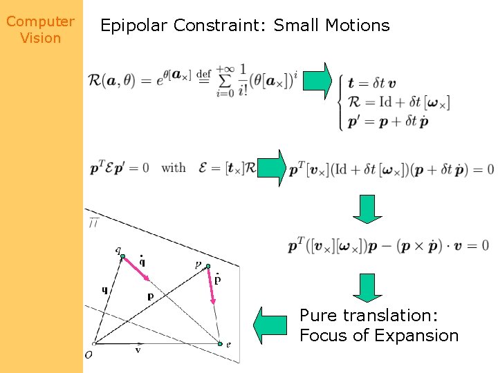
Computer Vision Epipolar Constraint: Small Motions To First-Order: Pure translation: Focus of Expansion

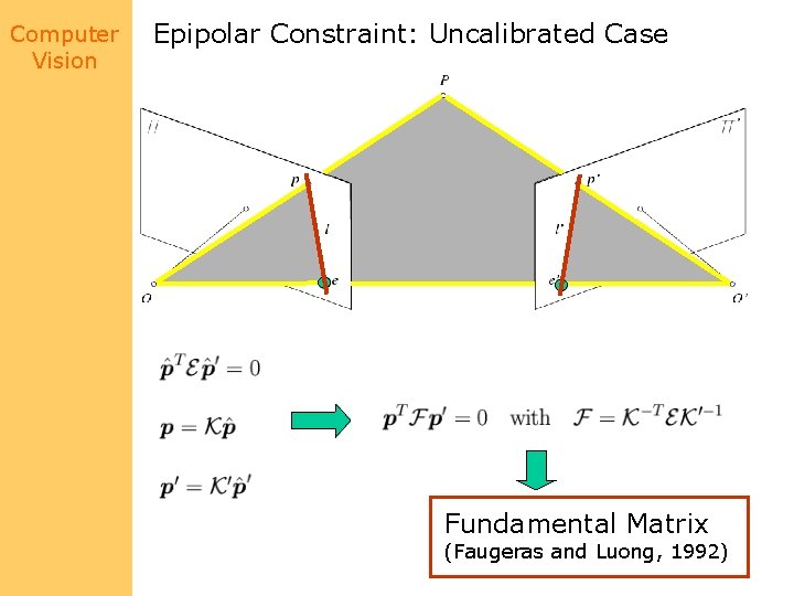
Computer Vision Epipolar Constraint: Uncalibrated Case Fundamental Matrix (Faugeras and Luong, 1992)

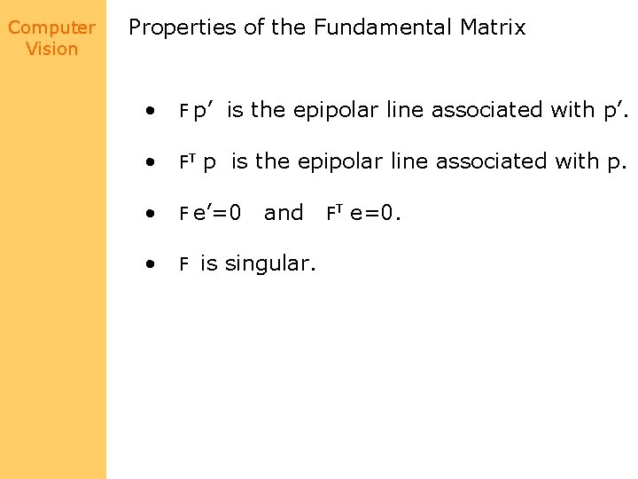
Properties of the Fundamental Matrix Computer Vision T • F p’ is the epipolar line associated with p’. • FT p is the epipolar line associated with p. T • F e’=0 • F is singular. and FT e=0.

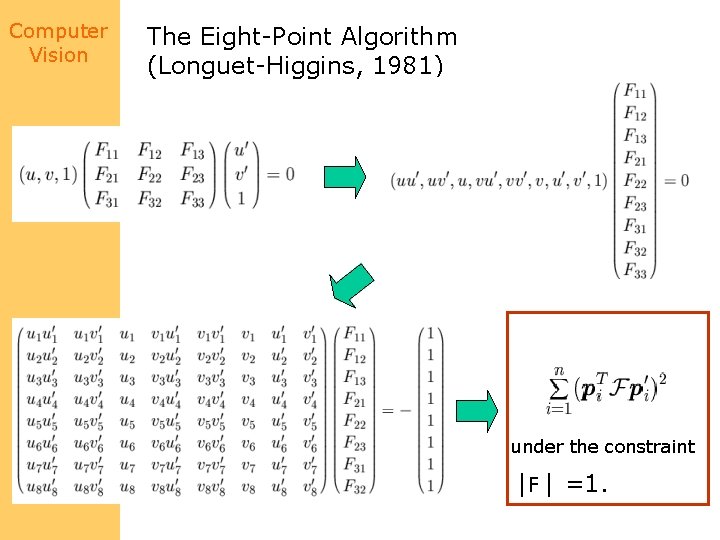
Computer Vision The Eight-Point Algorithm (Longuet-Higgins, 1981) Minimize: under the constraint |F |2 =1.

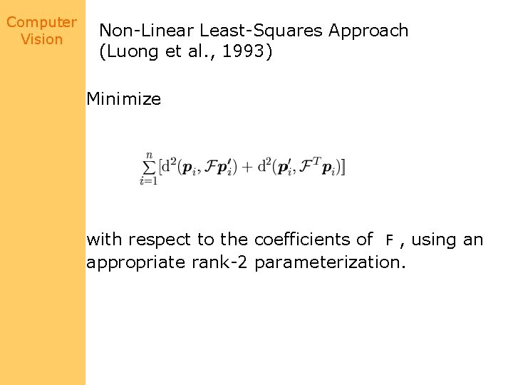
Computer Vision Non-Linear Least-Squares Approach (Luong et al. , 1993) Minimize with respect to the coefficients of F , using an appropriate rank-2 parameterization.

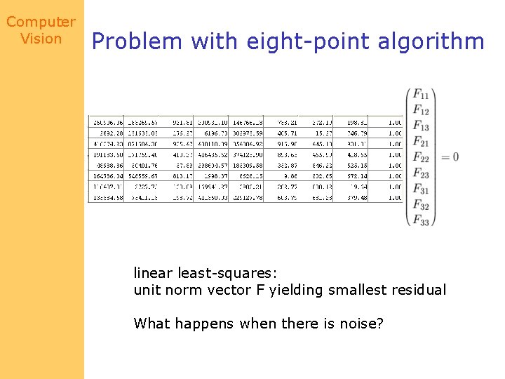
Computer Vision Problem with eight-point algorithm linear least-squares: unit norm vector F yielding smallest residual What happens when there is noise?

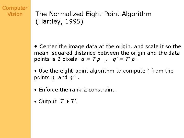
Computer Vision The Normalized Eight-Point Algorithm (Hartley, 1995) • Center the image data at the origin, and scale it so the mean squared distance between the origin and the data points is 2 pixels: q = T p , q’ = T’ p’. i i • Use the eight-point algorithm to compute F from the points q and q’. i i • Enforce the rank-2 constraint. • Output T F T’. T

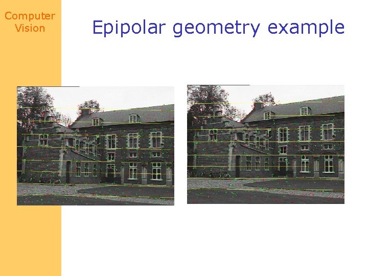
Computer Vision Epipolar geometry example

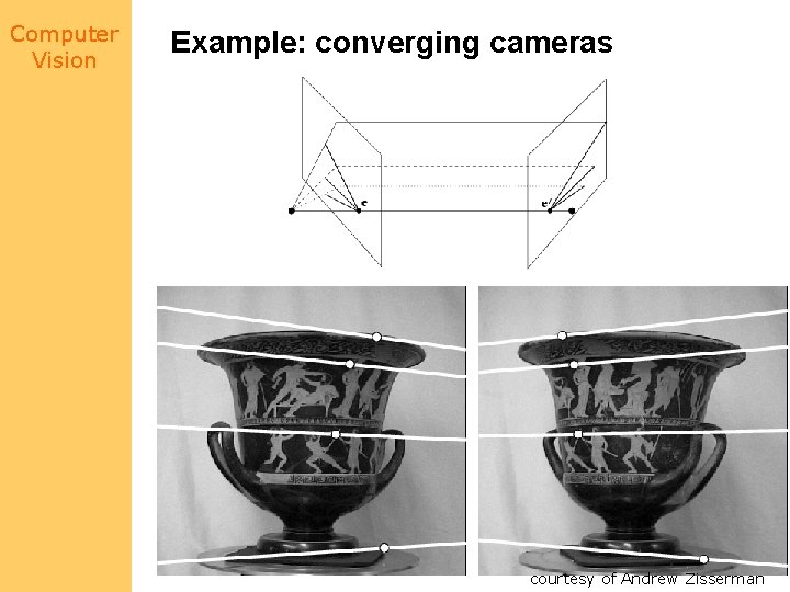
Computer Vision Example: converging cameras courtesy of Andrew Zisserman

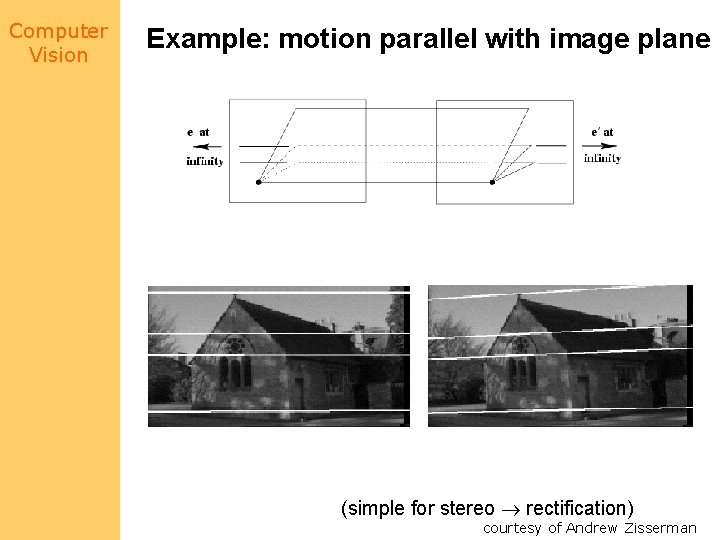
Computer Vision Example: motion parallel with image plane (simple for stereo rectification) courtesy of Andrew Zisserman

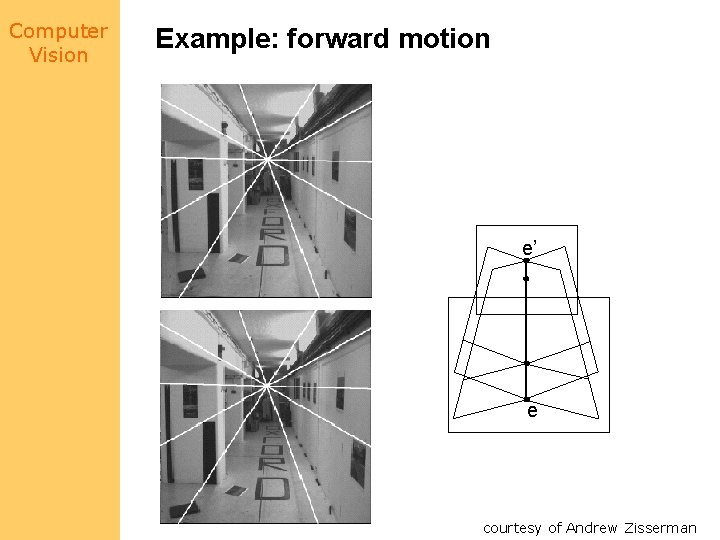
Computer Vision Example: forward motion e’ e courtesy of Andrew Zisserman

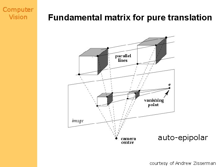
Computer Vision Fundamental matrix for pure translation auto-epipolar courtesy of Andrew Zisserman

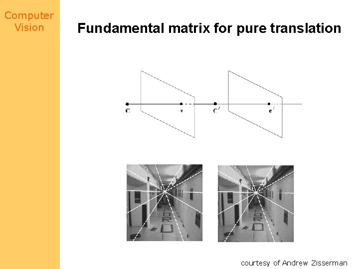
Computer Vision Fundamental matrix for pure translation courtesy of Andrew Zisserman

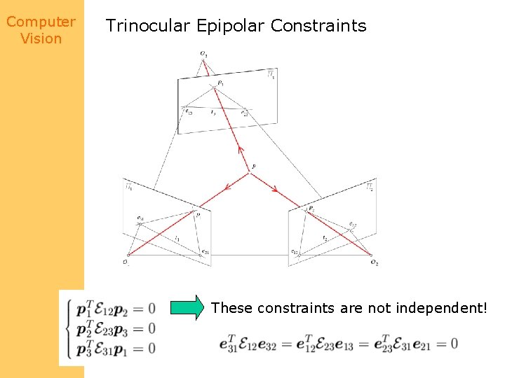
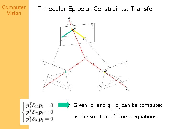
Computer Vision Trinocular Epipolar Constraints These constraints are not independent!

Computer Vision Trinocular Epipolar Constraints: Transfer Given p and p , p can be computed 1 2 3 as the solution of linear equations.

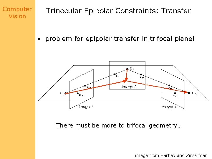
Computer Vision Trinocular Epipolar Constraints: Transfer • problem for epipolar transfer in trifocal plane! There must be more to trifocal geometry… image from Hartley and Zisserman

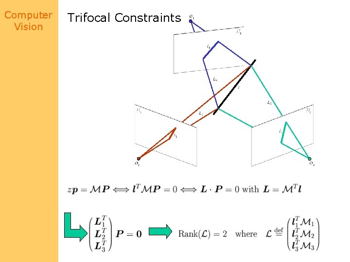
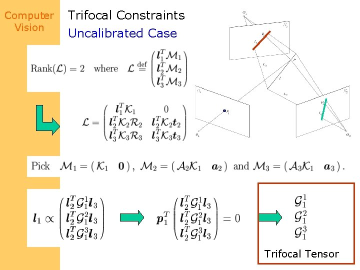
Computer Vision Trifocal Constraints

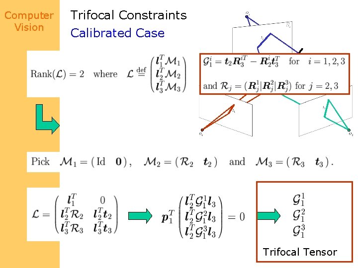
Computer Vision Trifocal Constraints Calibrated Case All 3 x 3 minors must be zero! Trifocal Tensor

Computer Vision Trifocal Constraints Uncalibrated Case Trifocal Tensor

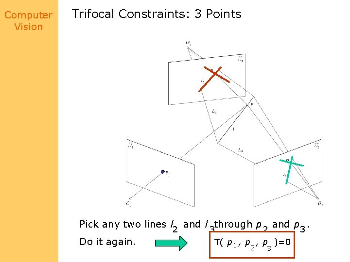
Computer Vision Trifocal Constraints: 3 Points Pick any two lines l 2 and l 3 through p 2 and p 3. Do it again. T( p 1 , p )=0 2 3

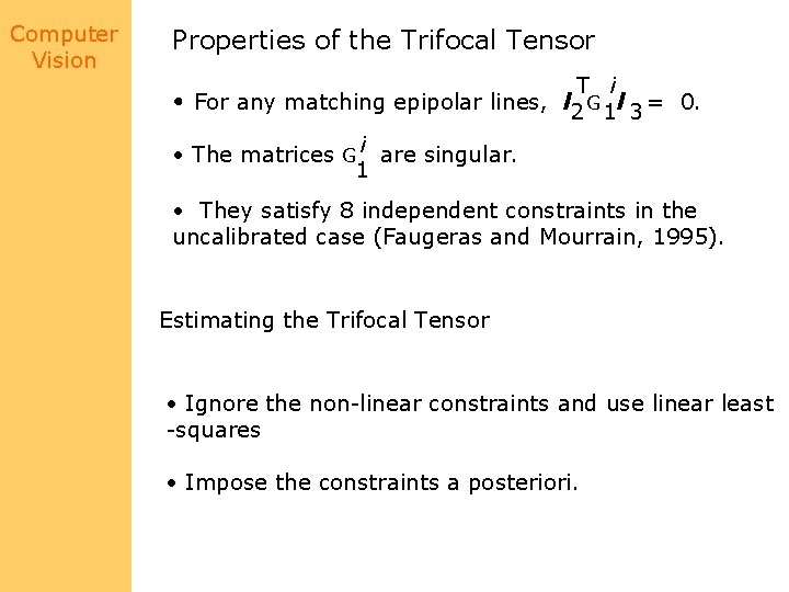
Computer Vision Properties of the Trifocal Tensor • For any matching epipolar lines, T i l 2 G 1 l 3 = 0. • The matrices G i are singular. 1 • They satisfy 8 independent constraints in the uncalibrated case (Faugeras and Mourrain, 1995). Estimating the Trifocal Tensor • Ignore the non-linear constraints and use linear least -squares • Impose the constraints a posteriori.

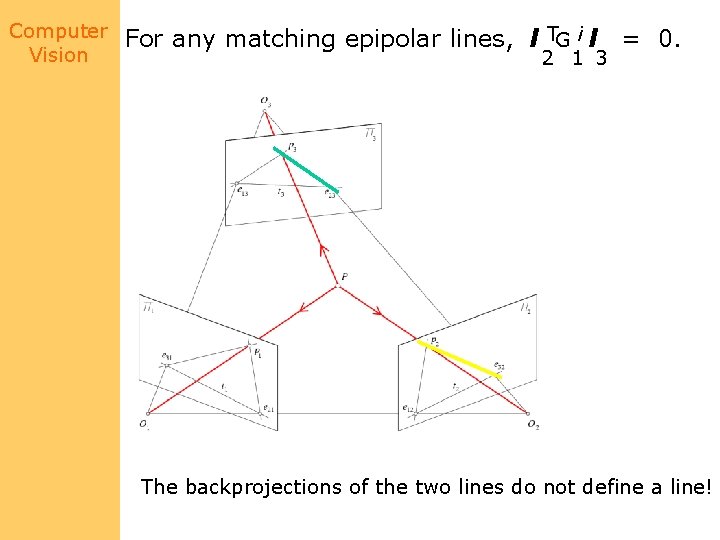
Computer Vision For any matching epipolar lines, l TG i l 2 1 3 = 0. The backprojections of the two lines do not define a line!

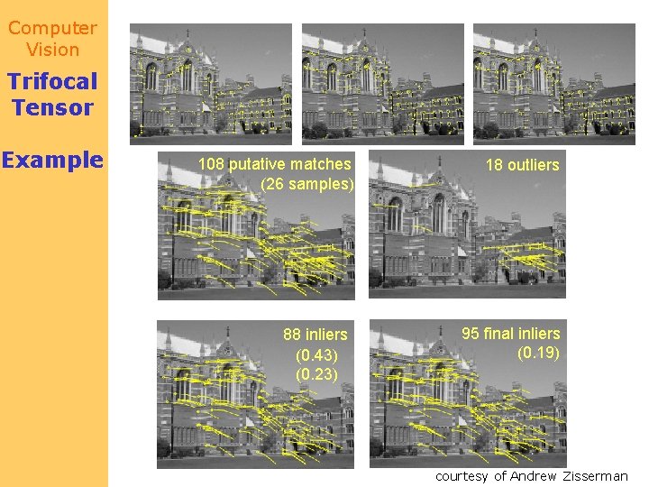
Computer Vision Trifocal Tensor Example 108 putative matches (26 samples) 88 inliers (0. 43) (0. 23) 18 outliers 95 final inliers (0. 19) courtesy of Andrew Zisserman

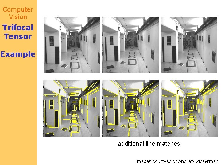
Computer Vision Trifocal Tensor Example additional line matches images courtesy of Andrew Zisserman

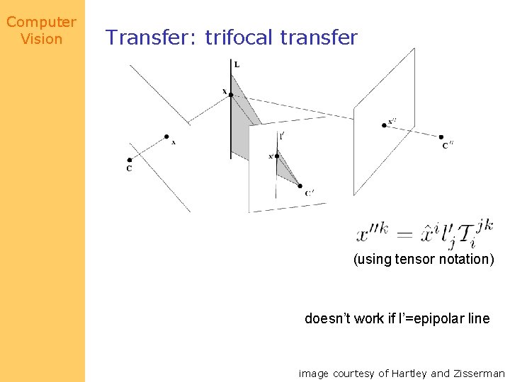
Computer Vision Transfer: trifocal transfer (using tensor notation) doesn’t work if l’=epipolar line image courtesy of Hartley and Zisserman

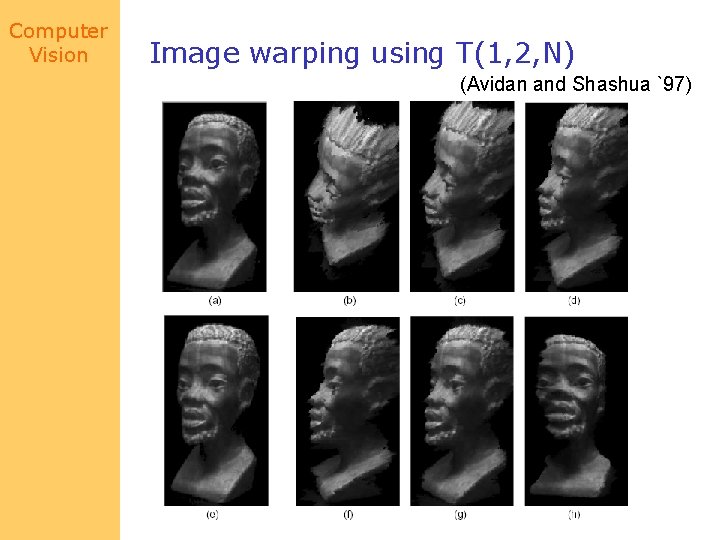
Computer Vision Image warping using T(1, 2, N) (Avidan and Shashua `97)

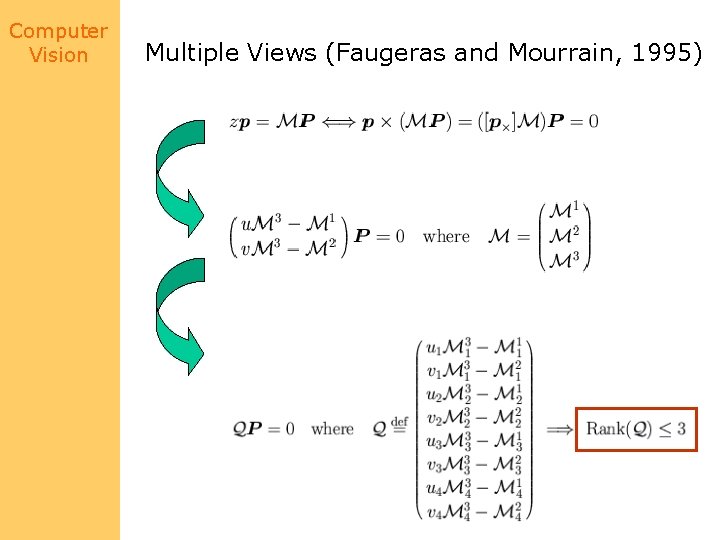
Computer Vision Multiple Views (Faugeras and Mourrain, 1995)

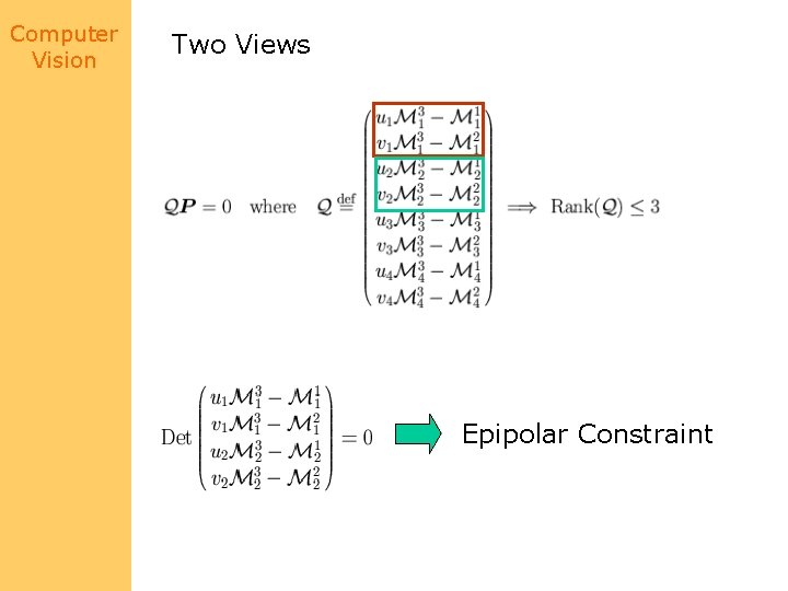
Computer Vision Two Views Epipolar Constraint

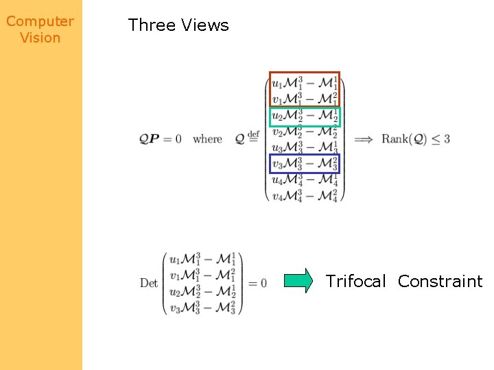
Computer Vision Three Views Trifocal Constraint

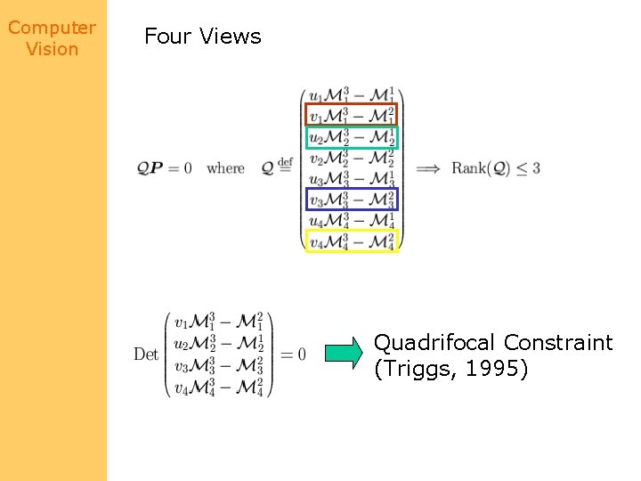
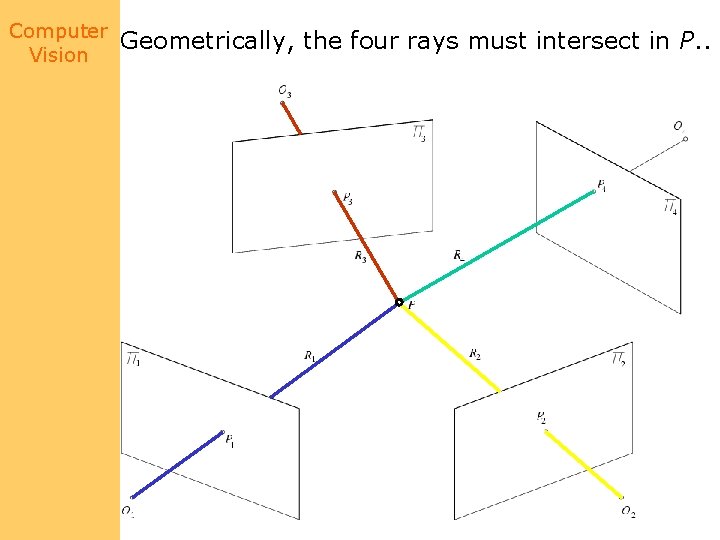
Computer Vision Four Views Quadrifocal Constraint (Triggs, 1995)

Computer Vision Geometrically, the four rays must intersect in P. .

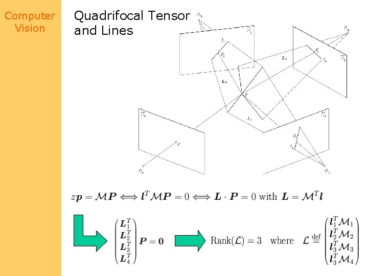
Computer Vision Quadrifocal Tensor and Lines

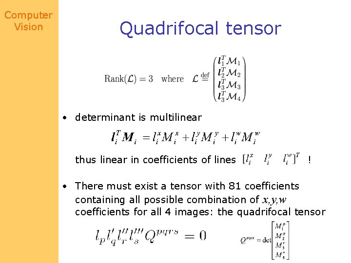
Computer Vision Quadrifocal tensor • determinant is multilinear thus linear in coefficients of lines ! • There must exist a tensor with 81 coefficients containing all possible combination of x, y, w coefficients for all 4 images: the quadrifocal tensor

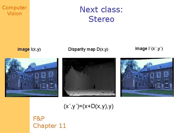
Computer Vision Next class: Stereo image I(x, y) Disparity map D(x, y) (x´, y´)=(x+D(x, y) F&P Chapter 11 image I´(x´, y´)