Multiple View Reconstruction Class 23 Multiple View Geometry

Multiple View Reconstruction Class 23 Multiple View Geometry Comp 290 -089 Marc Pollefeys

Administrivia • No papers to be presented • Probably take home exam

Content • Background: Projective geometry (2 D, 3 D), Parameter estimation, Algorithm evaluation. • Single View: Camera model, Calibration, Single View Geometry. • Two Views: Epipolar Geometry, 3 D reconstruction, Computing F, Computing structure, Plane and homographies. • Three Views: Trifocal Tensor, Computing T. • More Views: N-Linearities, Self-Calibration, Multi View Reconstruction, Bundle adjustment, Dynamic Sf. M, Cheirality, Duality

Multi-view computation

Multiple view computation • Tensors (2, 3, 4 -views) • Factorization • Orthographic • Perpective • Sequential • Bundle adjustment

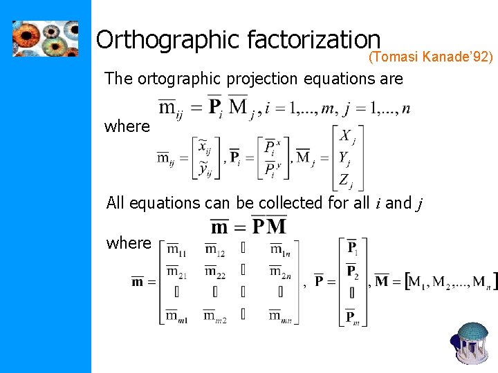
Orthographic factorization (Tomasi Kanade’ 92) The ortographic projection equations are where All equations can be collected for all i and j where

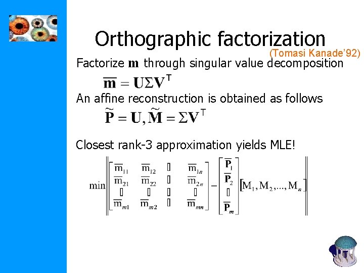
Orthographic factorization (Tomasi Kanade’ 92) Factorize m through singular value decomposition An affine reconstruction is obtained as follows Closest rank-3 approximation yields MLE!

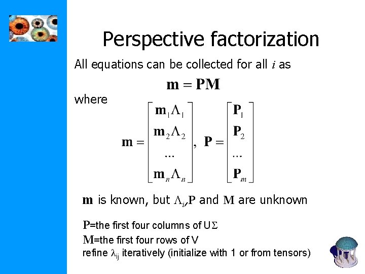
Perspective factorization All equations can be collected for all i as where m is known, but Li, P and M are unknown P=the first four columns of US M=the first four rows of V refine lij iteratively (initialize with 1 or from tensors)

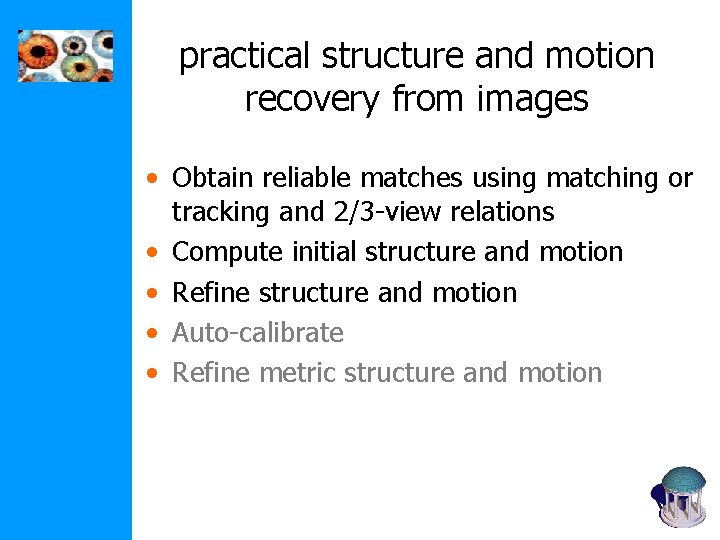
practical structure and motion recovery from images • Obtain reliable matches using matching or tracking and 2/3 -view relations • Compute initial structure and motion • Refine structure and motion • Auto-calibrate • Refine metric structure and motion

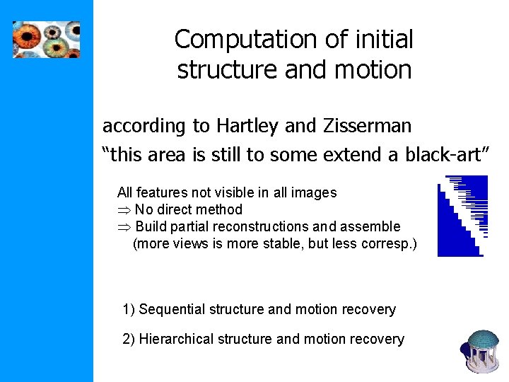
Computation of initial structure and motion according to Hartley and Zisserman “this area is still to some extend a black-art” All features not visible in all images Þ No direct method Þ Build partial reconstructions and assemble (more views is more stable, but less corresp. ) 1) Sequential structure and motion recovery 2) Hierarchical structure and motion recovery

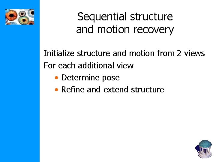
Sequential structure and motion recovery Initialize structure and motion from 2 views For each additional view • Determine pose • Refine and extend structure

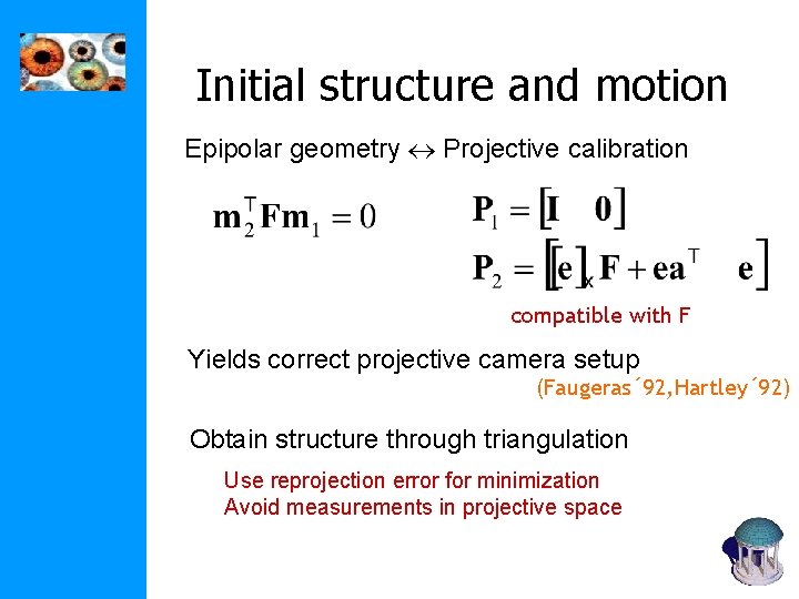
Initial structure and motion Epipolar geometry Projective calibration compatible with F Yields correct projective camera setup (Faugeras´ 92, Hartley´ 92) Obtain structure through triangulation Use reprojection error for minimization Avoid measurements in projective space

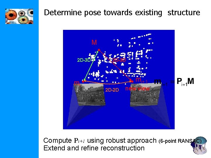
Determine pose towards existing structure M 2 D-3 D mi+1 2 D-2 D new view Compute Pi+1 using robust approach (6 -point RANSAC) Extend and refine reconstruction

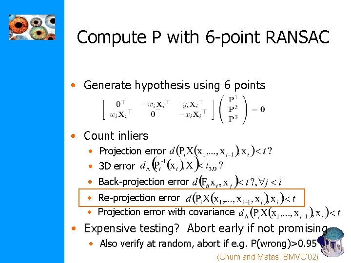
Compute P with 6 -point RANSAC • Generate hypothesis using 6 points • Count inliers • Projection error • 3 D error • Back-projection error • Re-projection error • Projection error with covariance • Expensive testing? Abort early if not promising • Also verify at random, abort if e. g. P(wrong)>0. 95 (Chum and Matas, BMVC’ 02)

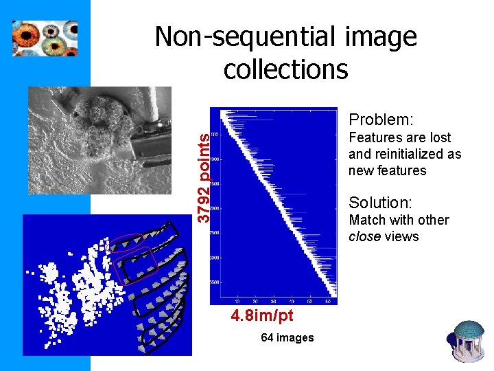
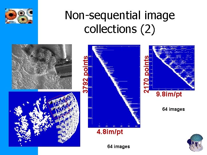
Non-sequential image collections Problem: 3792 points Features are lost and reinitialized as new features Solution: Match with other close views 4. 8 im/pt 64 images

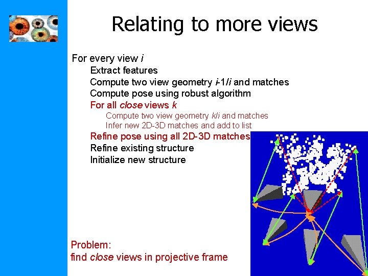
Relating to more views For every view i Extract features Compute two view geometry i-1/i and matches Compute pose using robust algorithm For all close views k Refine existing structure Compute view geometry k/i and matches Initialize newtwo structure Infer new 2 D-3 D matches and add to list Refine pose using all 2 D-3 D matches Refine existing structure Initialize new structure Problem: find close views in projective frame

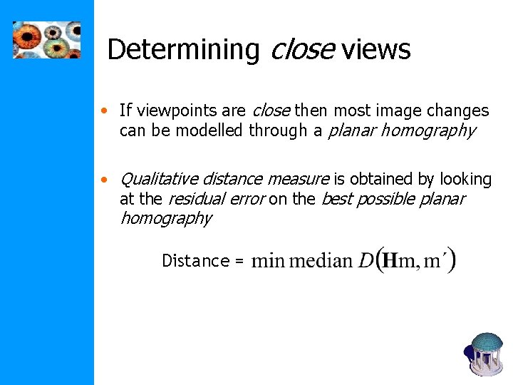
Determining close views • If viewpoints are close then most image changes can be modelled through a planar homography • Qualitative distance measure is obtained by looking at the residual error on the best possible planar homography Distance =

3792 points 2170 points Non-sequential image collections (2) 9. 8 im/pt 64 images 4. 8 im/pt 64 images

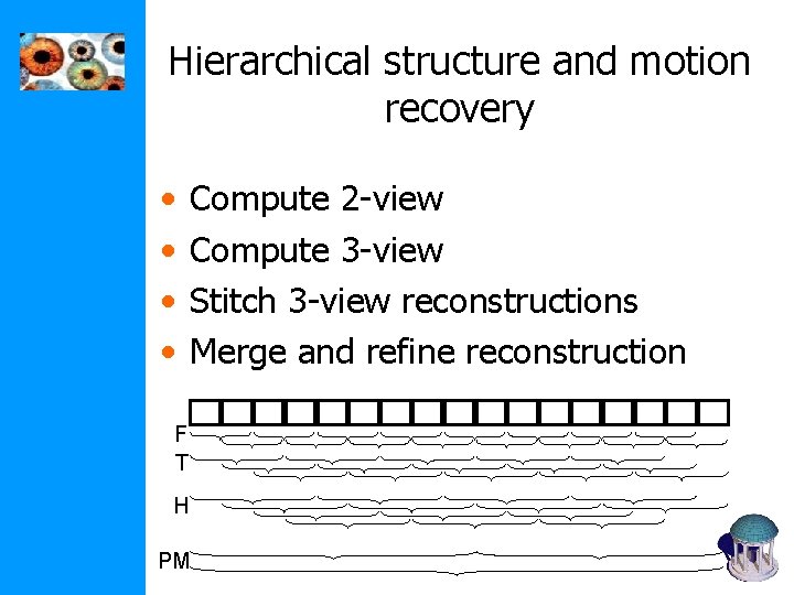
Hierarchical structure and motion recovery • • Compute 2 -view Compute 3 -view Stitch 3 -view reconstructions Merge and refine reconstruction F T H PM

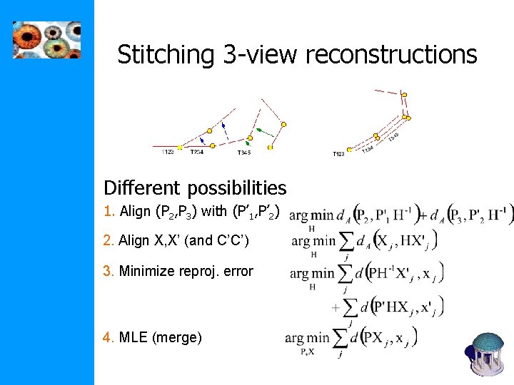
Stitching 3 -view reconstructions Different possibilities 1. Align (P 2, P 3) with (P’ 1, P’ 2) 2. Align X, X’ (and C’C’) 3. Minimize reproj. error 4. MLE (merge)

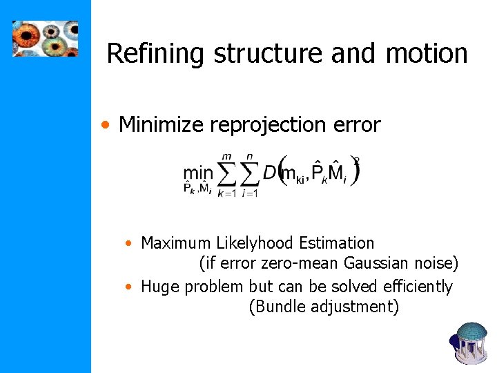
Refining structure and motion • Minimize reprojection error • Maximum Likelyhood Estimation (if error zero-mean Gaussian noise) • Huge problem but can be solved efficiently (Bundle adjustment)

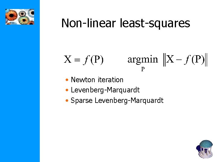
Non-linear least-squares • Newton iteration • Levenberg-Marquardt • Sparse Levenberg-Marquardt

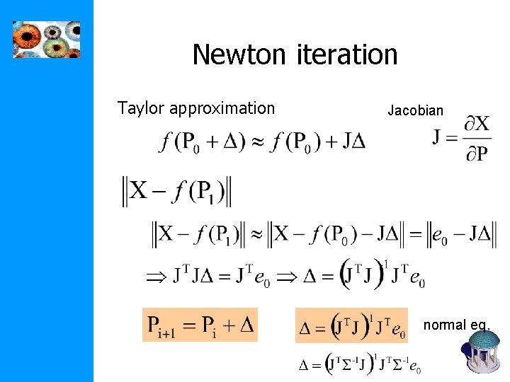
Newton iteration Taylor approximation Jacobian normal eq.

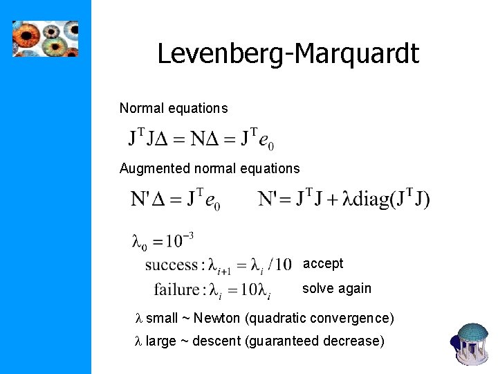
Levenberg-Marquardt Normal equations Augmented normal equations accept solve again l small ~ Newton (quadratic convergence) l large ~ descent (guaranteed decrease)

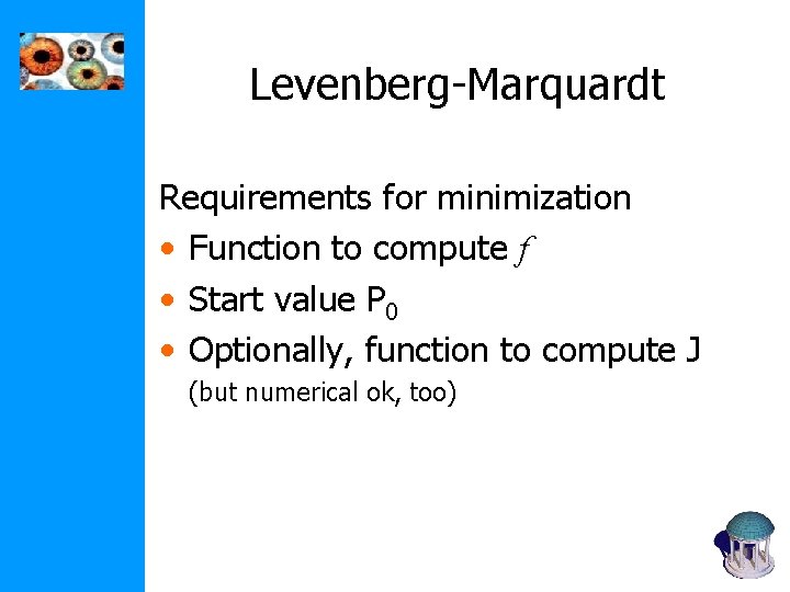
Levenberg-Marquardt Requirements for minimization • Function to compute f • Start value P 0 • Optionally, function to compute J (but numerical ok, too)

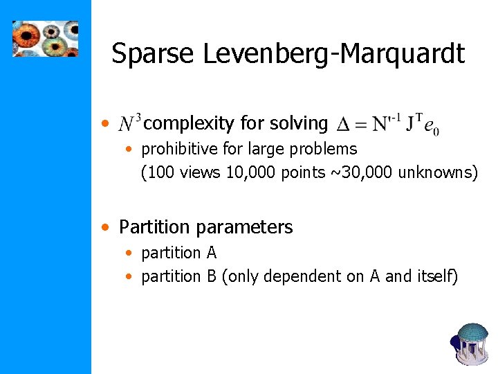
Sparse Levenberg-Marquardt • complexity for solving • prohibitive for large problems (100 views 10, 000 points ~30, 000 unknowns) • Partition parameters • partition A • partition B (only dependent on A and itself)

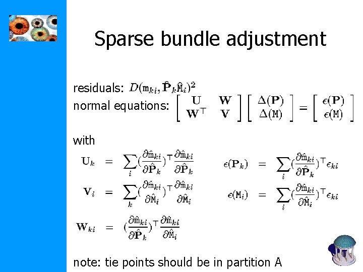
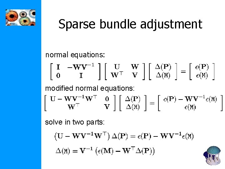
Sparse bundle adjustment residuals: normal equations: with note: tie points should be in partition A

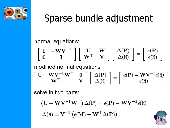
Sparse bundle adjustment normal equations: modified normal equations: solve in two parts:

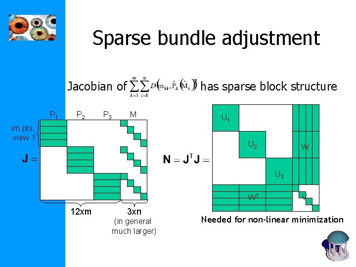
Sparse bundle adjustment Jacobian of P 1 P 2 P 3 has sparse block structure M im. pts. view 1 U 2 W U 3 WT 12 xm 3 xn (in general much larger) V Needed for non-linear minimization

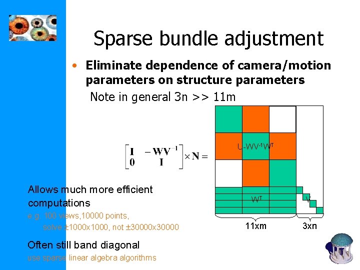
Sparse bundle adjustment • Eliminate dependence of camera/motion parameters on structure parameters Note in general 3 n >> 11 m U-WV-1 WT Allows much more efficient computations e. g. 100 views, 10000 points, solve 1000 x 1000, not 30000 x 30000 Often still band diagonal use sparse linear algebra algorithms WT V 11 xm 3 xn

Sparse bundle adjustment normal equations: modified normal equations: solve in two parts:

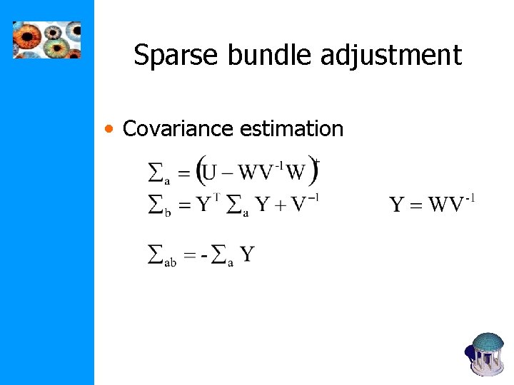
Sparse bundle adjustment • Covariance estimation

Next class: Dynamic structure from motion