Computer Architecture A Quantitative Approach Sixth Edition Chapter

Computer Architecture A Quantitative Approach, Sixth Edition Chapter 7 Domain-Specific Architectures Copyright © 2019, Elsevier Inc. All rights Reserved 1

n Moore’s Law enabled: n n n n n Introduction Deep memory hierarchy Wide SIMD units Deep pipelines Branch prediction Out-of-order execution Speculative prefetching Multithreading Multiprocessing Objective: n Extract performance from software that is oblivious to architecture Copyright © 2019, Elsevier Inc. All rights Reserved 2

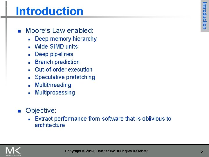
Figure 7. 1 Time before new Intel semiconductor process technology measured in nm. The y-axis is log scale. Note that the time stretched previously from about 24 months per new process step to about 30 months since 2010. 3

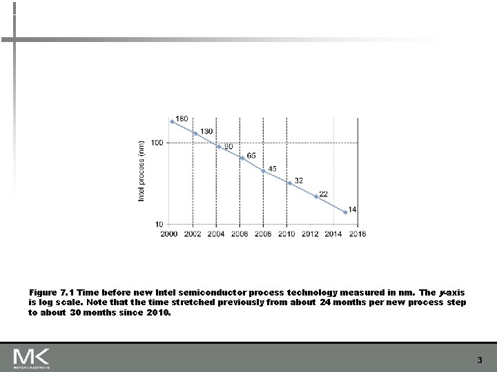
n Need factor of 100 improvements in number of operations per instruction n Introduction Requires domain specific architectures For ASICs, NRE cannot be amoratized over large volumes FPGAs are less efficient than ASICs Copyright © 2019, Elsevier Inc. All rights Reserved 4

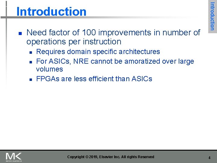
Figure 7. 2 Energy costs in pico. Joules for a 90 nm process to fetch instructions or access a data cache compared to the energy cost of arithmetic operations (Qadeer et al. , 2015). This slide is a strong argument for DSAs 5

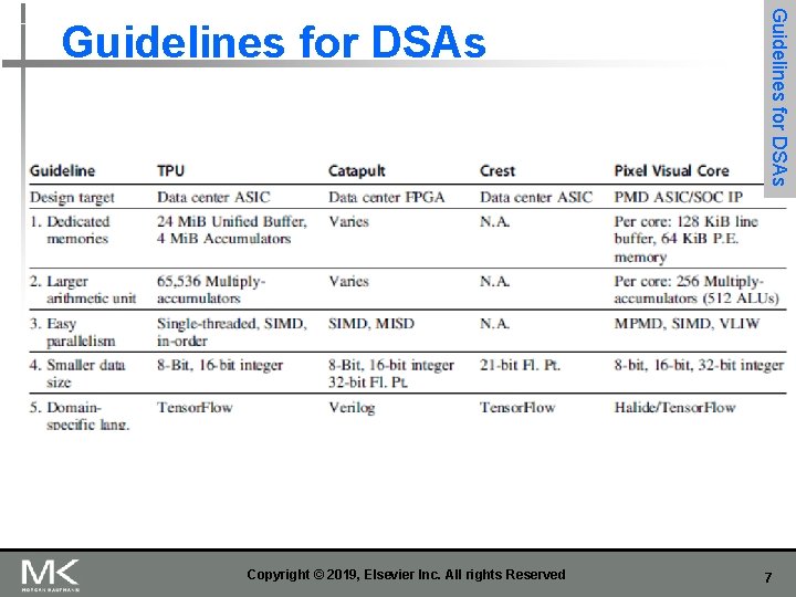
n n n n Use dedicated memories to minimize data movement Invest resources into more arithmetic units or bigger memories Use the easiest form of parallelism that matches the domain Reduce data size and type to the simplest needed for the domain Use a domain-specific programming language Guidelines for DSAs Per text in HP 19: domain-specific algorithms are always for small compute intensive kernels of large programs; DSAs are unlikely for large C++ SPEC 2017 programs (e. g. , compiler) Architects need to expand their expertise for DSAs Copyright © 2019, Elsevier Inc. All rights Reserved 6

Copyright © 2019, Elsevier Inc. All rights Reserved Guidelines for DSAs 7

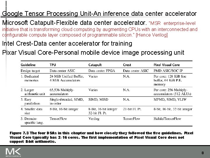
Google Tensor Processing Unit-An inference data center accelerator Microsoft Catapult-Flexible data center accelerator. “MSR enterprise-level initiative that is transforming cloud computing by augmenting CPUs with an interconnected and configurable compute layer composed of programmable silicon. ” [Hence Verilog] Intel Crest-Data center accelerator for training Pixar Visual Core-Personal mobile device image processing unit Figure 7. 3 The four DSAs in this chapter and how closely they followed the five guidelines. Pixel Visual Core typically has 2– 16 cores. The first implementation of Pixel Visual Core does not support 8 -bit arithmetic. 8

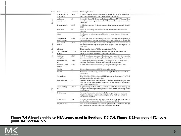
Figure 7. 4 A handy guide to DSA terms used in Sections 7. 3– 7. 6. Figure 7. 29 on page 472 has a guide for Section 7. 7. 9

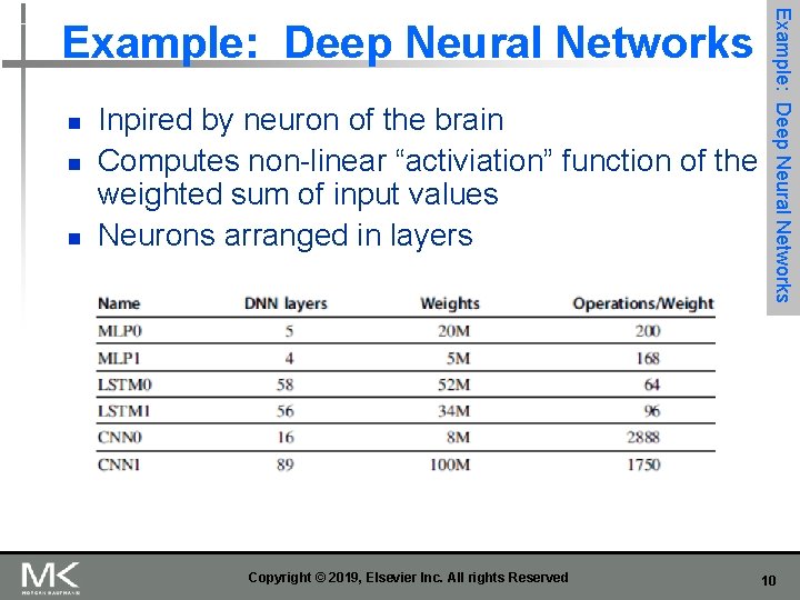
n n n Inpired by neuron of the brain Computes non-linear “activiation” function of the weighted sum of input values Neurons arranged in layers Copyright © 2019, Elsevier Inc. All rights Reserved Example: Deep Neural Networks 10

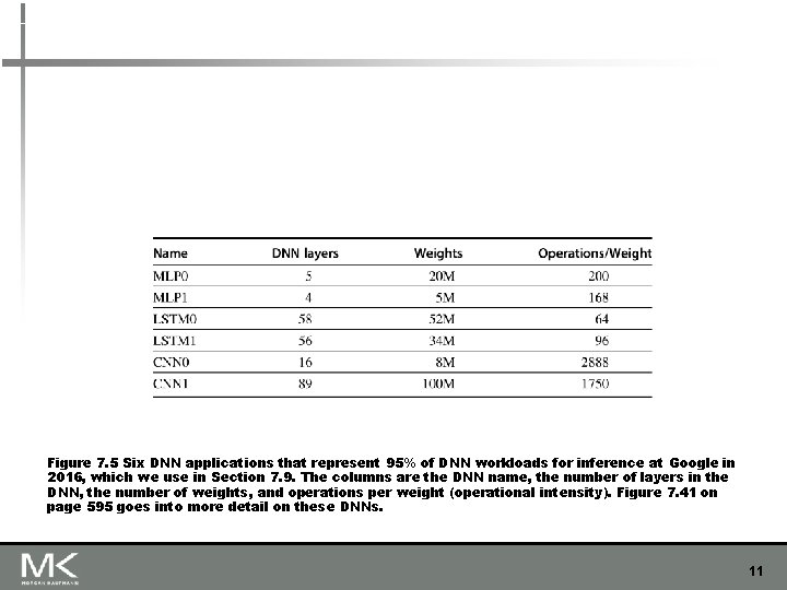
Figure 7. 5 Six DNN applications that represent 95% of DNN workloads for inference at Google in 2016, which we use in Section 7. 9. The columns are the DNN name, the number of layers in the DNN, the number of weights, and operations per weight (operational intensity). Figure 7. 41 on page 595 goes into more detail on these DNNs. 11

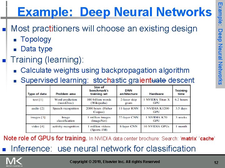
Example: Deep Neural Networks n Most practitioners will choose an existing design n Topology Data type Training (learning): n n Calculate weights using backpropagation algorithm Supervised learning: stochastic graientuate descent Note role of GPUs for training. In NVIDIA data center brochure: Search: ‘matrix’ ‘cache’ n Inferrence: use neural network for classification Copyright © 2019, Elsevier Inc. All rights Reserved 12

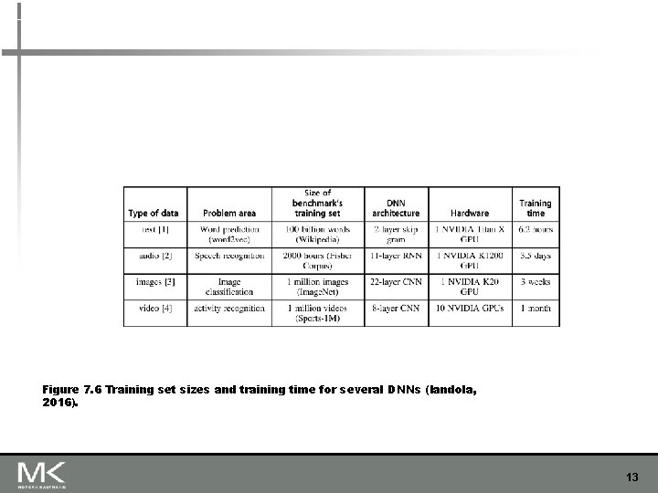
Figure 7. 6 Training set sizes and training time for several DNNs (Iandola, 2016). 13

n Parameters: n n n Dim[i]: number of neurons Dim[i-1]: dimension of input vector Number of weights: Dim[i-1] x Dim[i] Operations: 2 x Dim[i-1] x Dim[i] Operations/weight: 2 Copyright © 2019, Elsevier Inc. All rights Reserved Example: Deep Neural Networks Multi-Layer Perceptrons 14

Figure 7. 7 MLP showing the input Layer[ i− 1] on the left and the output Layer[ i] on the right. Re. LU is a popular nonlinear function for MLPs. The dimensions of the input and output layers are often different. Such a layer is called fully connected because it depends on all the inputs from the prior layer, even if many of them are zeros. One study suggested that 44% were zeros, which presumably is in part because Re. LU turns negative numbers into zeros. 15

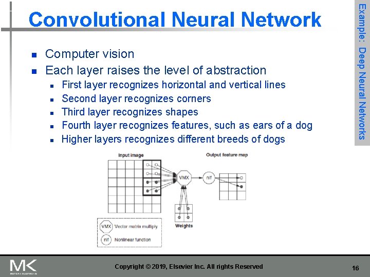
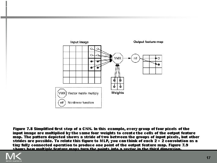
n n Computer vision Each layer raises the level of abstraction n n First layer recognizes horizontal and vertical lines Second layer recognizes corners Third layer recognizes shapes Fourth layer recognizes features, such as ears of a dog Higher layers recognizes different breeds of dogs Copyright © 2019, Elsevier Inc. All rights Reserved Example: Deep Neural Networks Convolutional Neural Network 16

Figure 7. 8 Simplified first step of a CNN. In this example, every group of four pixels of the input image are multiplied by the same four weights to create the cells of the output feature map. The pattern depicted shows a stride of two between the groups of input pixels, but other strides are possible. To relate this figure to MLP, you can think of each 2 × 2 convolution as a tiny fully connected operation to produce one point of the output feature map. Figure 7. 9 shows how multiple feature maps turn the points into a vector in the third dimension. 17

n Parameters: n n n Example: Deep Neural Networks Convolutional Neural Network Dim. FM[i-1]: Dimension of the (square) input Feature Map Dim. FM[i]: Dimension of the (square) output Feature Map Dim. Sten[i]: Dimension of the (square) stencil Num. FM[i-1]: Number of input Feature Maps Num. FM[i]: Number of output Feature Maps Number of neurons: Num. FM[i] x Dim. FM[i]2 Number of weights per output Feature Map: Num. FM[i-1] x Dim. Sten[i]2 Total number of weights per layer: Num. FM[i] x Number of weights per output Feature Map Number of operations per output Feature Map: 2 x Dim. FM[i]2 x Number of weights per output Feature Map Total number of operations per layer: Num. FM[i] x Number of operations per output Feature Map = 2 x Dim. FM[i]2 x Num. FM[i] x Number of weights per output Feature Map = 2 x Dim. FM[i]2 x Total number of weights per layer Operations/Weight: 2 x Dim. FM[i]2 Copyright © 2019, Elsevier Inc. All rights Reserved 18

Figure 7. 9 CNN general step showing input feature maps of Layer[ i− 1] on the left, the output feature maps of Layer[i] on the right, and a three-dimensional stencil over input feature maps to produce a single output feature map. Each output feature map has its own unique set of weights, and the vector-matrix multiply happens for every one. The dotted lines show future output feature maps in this figure. As this figure illustrates, the dimensions and number of the input and output feature maps are often different. As with MLPs, Re. LU is a popular nonlinear function for CNNs. 19

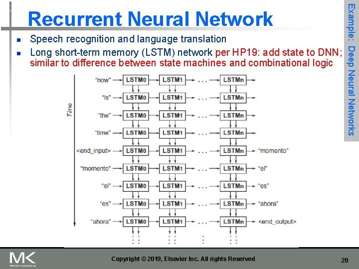
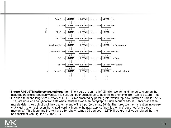
n n Speech recognition and language translation Long short-term memory (LSTM) network per HP 19: add state to DNN; similar to difference between state machines and combinational logic Copyright © 2019, Elsevier Inc. All rights Reserved Example: Deep Neural Networks Recurrent Neural Network 20

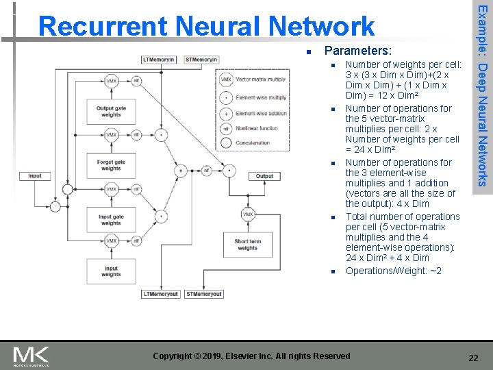
Figure 7. 10 LSTM cells connected together. The inputs are on the left (English words), and the outputs are on the right (the translated Spanish words). The cells can be thought of as being unrolled over time, from top to bottom. Thus the short-term and long-term memory of LSTM is implemented by passing information top-down between unrolled cells. They are unrolled enough to translate whole sentences or even paragraphs. Such sequence-to-sequence translation models delay their output until they get to the end of the input (Wu et al. , 2016). They produce the translation in reverse order, using the most recent translated word as input to the next step, so “now is the time” becomes “ahora es el momento. ” (This figure and the next are often shown turned 90 degrees in LSTM literature, but we’ve rotated them to be consistent with Figures 7. 7 and 7. 8. ) 21

n Parameters: n n n Number of weights per cell: 3 x (3 x Dim)+(2 x Dim) + (1 x Dim) = 12 x Dim 2 Number of operations for the 5 vector-matrix multiplies per cell: 2 x Number of weights per cell = 24 x Dim 2 Number of operations for the 3 element-wise multiplies and 1 addition (vectors are all the size of the output): 4 x Dim Total number of operations per cell (5 vector-matrix multiplies and the 4 element-wise operations): 24 x Dim 2 + 4 x Dim Operations/Weight: ~2 Copyright © 2019, Elsevier Inc. All rights Reserved Example: Deep Neural Networks Recurrent Neural Network 22

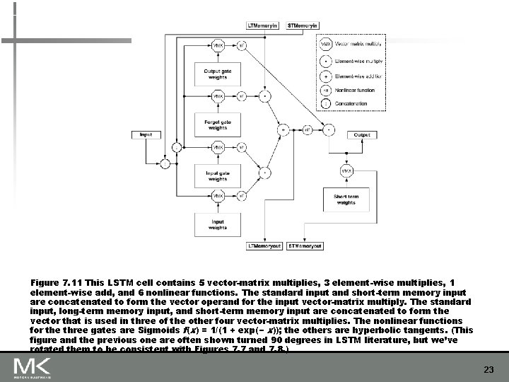
Figure 7. 11 This LSTM cell contains 5 vector-matrix multiplies, 3 element-wise multiplies, 1 element-wise add, and 6 nonlinear functions. The standard input and short-term memory input are concatenated to form the vector operand for the input vector-matrix multiply. The standard input, long-term memory input, and short-term memory input are concatenated to form the vector that is used in three of the other four vector-matrix multiplies. The nonlinear functions for the three gates are Sigmoids f(x) = 1/(1 + exp(− x)); the others are hyperbolic tangents. (This figure and the previous one are often shown turned 90 degrees in LSTM literature, but we’ve rotated them to be consistent with Figures 7. 7 and 7. 8. ) 23

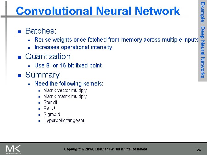
n Batches: n n n Quantization n n Reuse weights once fetched from memory across multiple inputs Increases operational intensity Use 8 - or 16 -bit fixed point Summary: n Example: Deep Neural Networks Convolutional Neural Network Need the following kernels: n n n Matrix-vector multiply Matrix-matrix multiply Stencil Re. LU Sigmoid Hyperbolic tangeant Copyright © 2019, Elsevier Inc. All rights Reserved 24

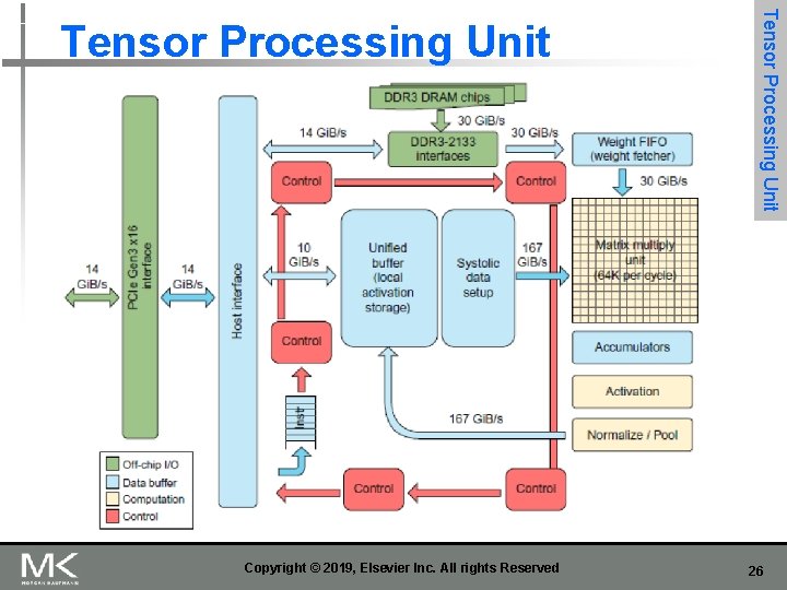
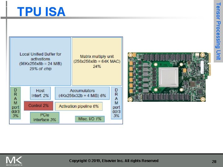
n n Google’s DNN ASIC 256 x 256 8 -bit matrix multiply unit Large software-managed scratchpad Coprocessor on the PCIe bus Copyright © 2019, Elsevier Inc. All rights Reserved Tensor Processing Unit 25

Copyright © 2019, Elsevier Inc. All rights Reserved Tensor Processing Unit 26

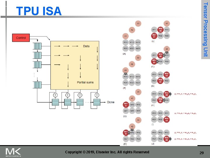
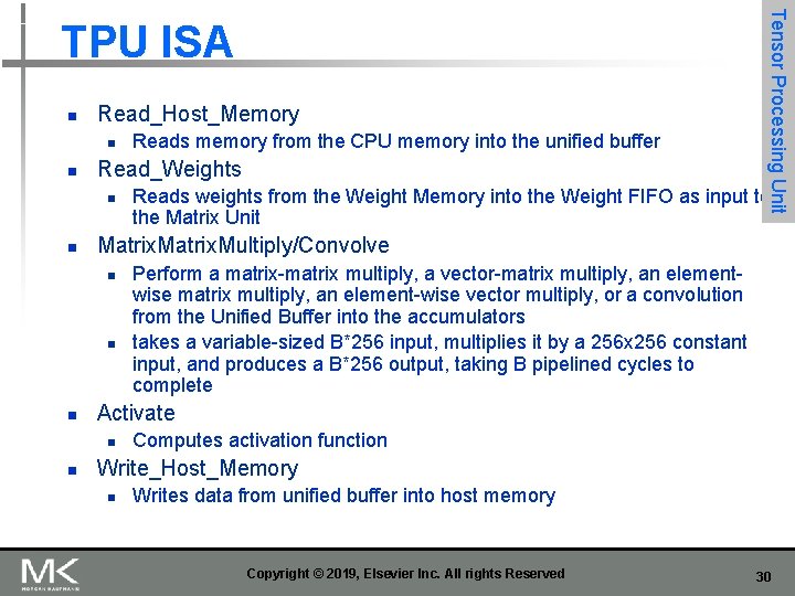
n Read_Host_Memory n n Read_Weights n n n Perform a matrix-matrix multiply, a vector-matrix multiply, an elementwise matrix multiply, an element-wise vector multiply, or a convolution from the Unified Buffer into the accumulators takes a variable-sized B*256 input, multiplies it by a 256 x 256 constant input, and produces a B*256 output, taking B pipelined cycles to complete Activate n n Reads weights from the Weight Memory into the Weight FIFO as input to the Matrix Unit Matrix. Multiply/Convolve n n Reads memory from the CPU memory into the unified buffer Tensor Processing Unit TPU ISA Computes activation function Write_Host_Memory n Writes data from unified buffer into host memory Copyright © 2019, Elsevier Inc. All rights Reserved 27

Tensor Processing Unit TPU ISA Copyright © 2019, Elsevier Inc. All rights Reserved 28

Tensor Processing Unit TPU ISA Copyright © 2019, Elsevier Inc. All rights Reserved 29

n Read_Host_Memory n n Read_Weights n n n Perform a matrix-matrix multiply, a vector-matrix multiply, an elementwise matrix multiply, an element-wise vector multiply, or a convolution from the Unified Buffer into the accumulators takes a variable-sized B*256 input, multiplies it by a 256 x 256 constant input, and produces a B*256 output, taking B pipelined cycles to complete Activate n n Reads weights from the Weight Memory into the Weight FIFO as input to the Matrix Unit Matrix. Multiply/Convolve n n Reads memory from the CPU memory into the unified buffer Tensor Processing Unit TPU ISA Computes activation function Write_Host_Memory n Writes data from unified buffer into host memory Copyright © 2019, Elsevier Inc. All rights Reserved 30

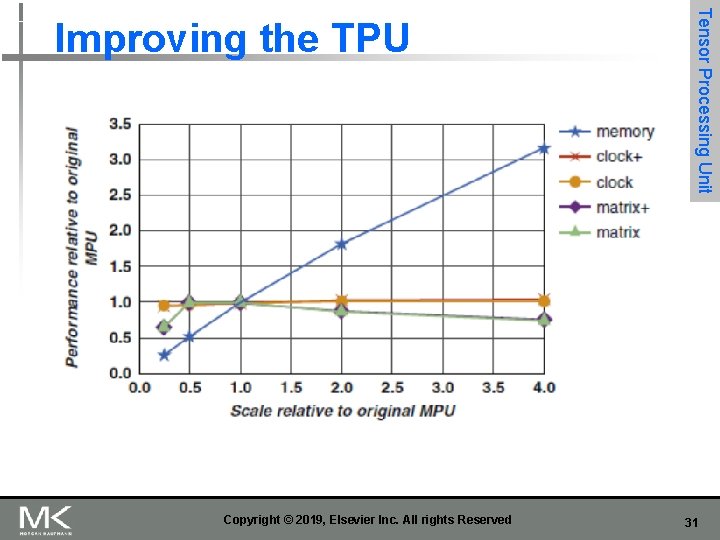
Copyright © 2019, Elsevier Inc. All rights Reserved Tensor Processing Unit Improving the TPU 31

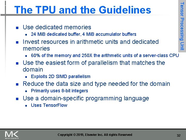
Tensor Processing Unit The TPU and the Guidelines n Use dedicated memories n n Invest resources in arithmetic units and dedicated memories n n Exploits 2 D SIMD parallelism Reduce the data size and type needed for the domain n n 60% of the memory and 250 X the arithmetic units of a server-class CPU Use the easiest form of parallelism that matches the domain n n 24 Mi. B dedicated buffer, 4 Mi. B accumulator buffers Primarily uses 8 -bit integers Use a domain-specific programming language n Uses Tensor. Flow Copyright © 2019, Elsevier Inc. All rights Reserved 32

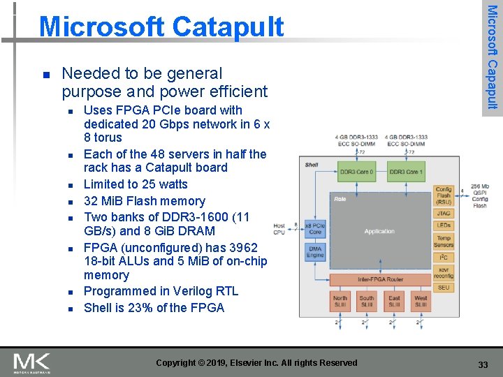
n Needed to be general purpose and power efficient n n n n Uses FPGA PCIe board with dedicated 20 Gbps network in 6 x 8 torus Each of the 48 servers in half the rack has a Catapult board Limited to 25 watts 32 Mi. B Flash memory Two banks of DDR 3 -1600 (11 GB/s) and 8 Gi. B DRAM FPGA (unconfigured) has 3962 18 -bit ALUs and 5 Mi. B of on-chip memory Programmed in Verilog RTL Shell is 23% of the FPGA Copyright © 2019, Elsevier Inc. All rights Reserved Microsoft Capapult Microsoft Catapult 33

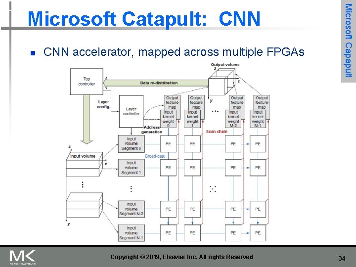
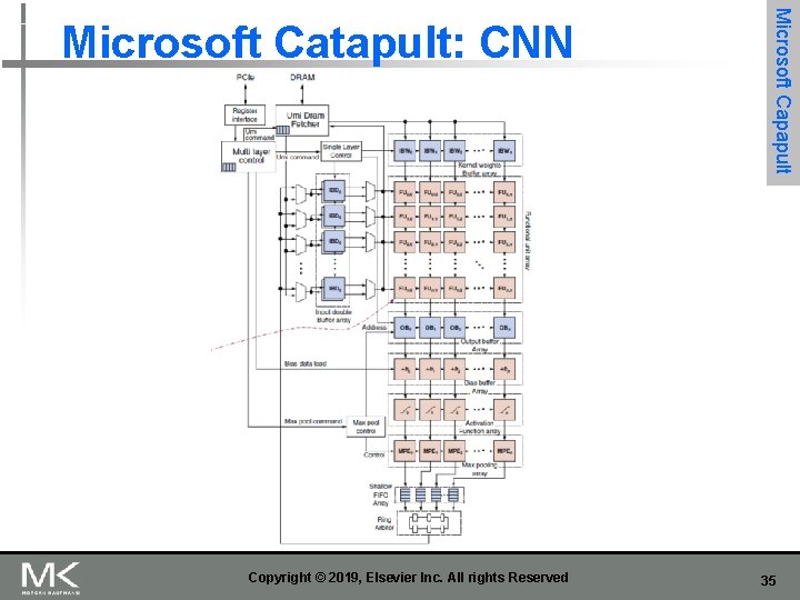
n CNN accelerator, mapped across multiple FPGAs Copyright © 2019, Elsevier Inc. All rights Reserved Microsoft Capapult Microsoft Catapult: CNN 34

Copyright © 2019, Elsevier Inc. All rights Reserved Microsoft Capapult Microsoft Catapult: CNN 35

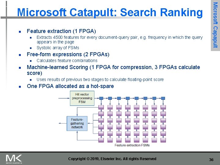
n Feature extraction (1 FPGA) n n n Free-form expressions (2 FPGAs) n n Calculates feature combinations Machine-learned Scoring (1 FPGA for compression, 3 FPGAs calculate score) n n Extracts 4500 features for every document-query pair, e. g. frequency in which the query appears in the page Systolic array of FSMs Microsoft Capapult Microsoft Catapult: Search Ranking Uses results of previous two stages to calculate floating-point score One FPGA allocated as a hot-spare Copyright © 2019, Elsevier Inc. All rights Reserved 36

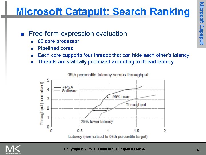
n Free-form expression evaluation n n 60 core processor Pipelined cores Each core supports four threads that can hide each other’s latency Threads are statically prioritized according to thread latency Copyright © 2019, Elsevier Inc. All rights Reserved Microsoft Capapult Microsoft Catapult: Search Ranking 37

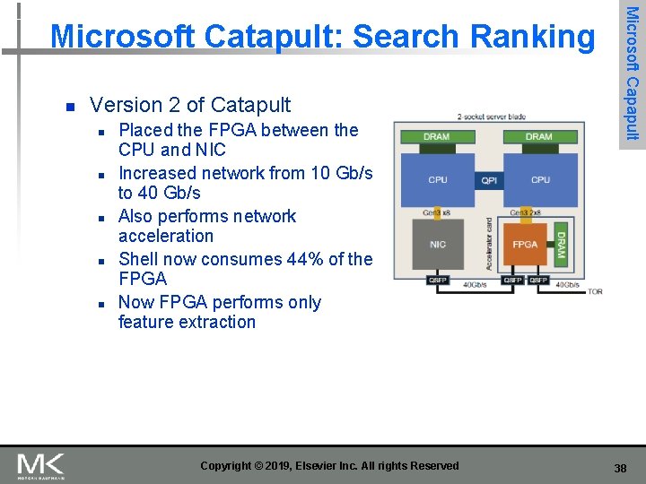
n Version 2 of Catapult n n n Placed the FPGA between the CPU and NIC Increased network from 10 Gb/s to 40 Gb/s Also performs network acceleration Shell now consumes 44% of the FPGA Now FPGA performs only feature extraction Copyright © 2019, Elsevier Inc. All rights Reserved Microsoft Capapult Microsoft Catapult: Search Ranking 38

n Use dedicated memories n n Invest resources in arithmetic units and dedicated memories n n 2 D SIMD for CNN, MISD parallelism for search scoring Reduce the data size and type needed for the domain n n 3926 ALUs Use the easiest form of parallelism that matches the domain n n 5 Mi. B dedicated memory Microsoft Capapult Catapult and the Guidelines Uses mixture of 8 -bit integers and 64 -bit floating-point Use a domain-specific programming language n Uses Verilog RTL; Microsoft did not follow this guideline Copyright © 2019, Elsevier Inc. All rights Reserved 39

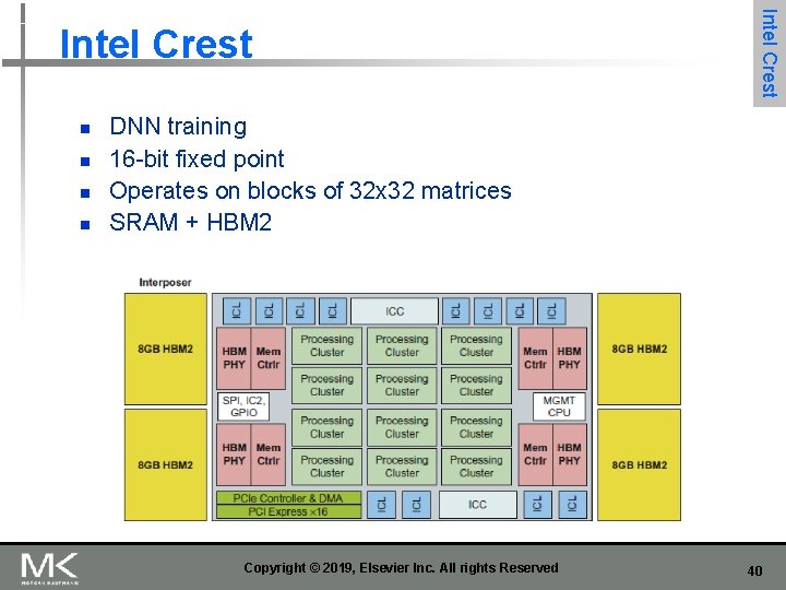
n n Intel Crest DNN training 16 -bit fixed point Operates on blocks of 32 x 32 matrices SRAM + HBM 2 Copyright © 2019, Elsevier Inc. All rights Reserved 40

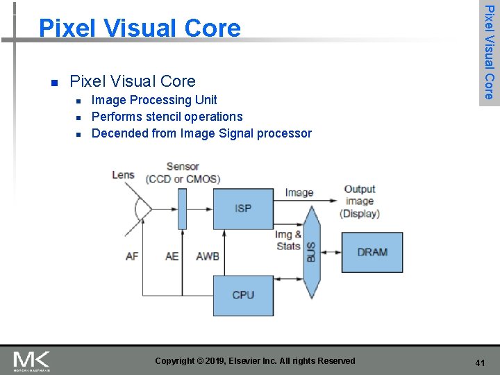
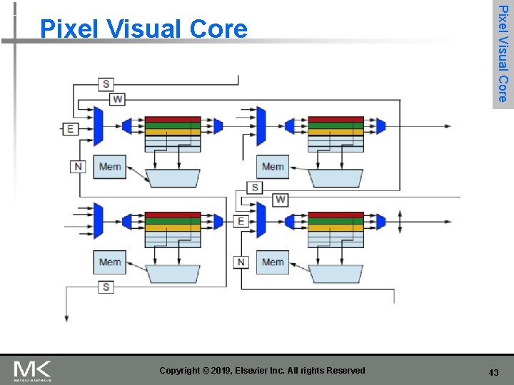
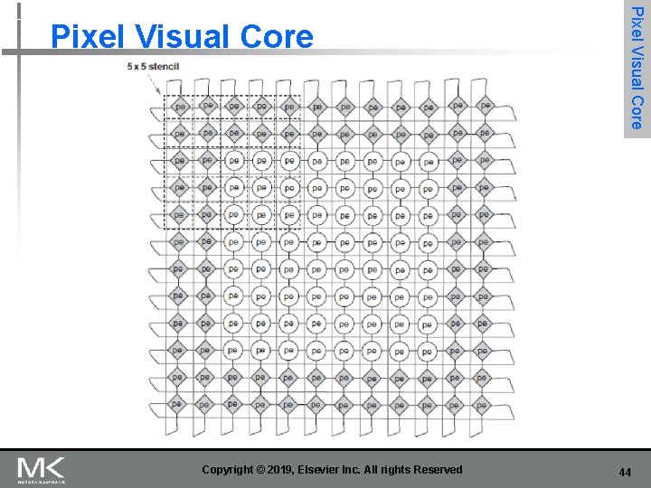
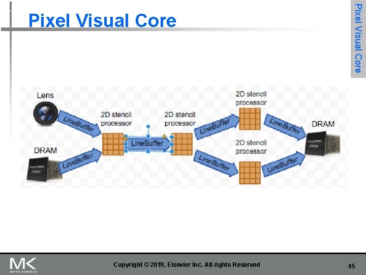
n Pixel Visual Core n n n Image Processing Unit Performs stencil operations Decended from Image Signal processor Copyright © 2019, Elsevier Inc. All rights Reserved Pixel Visual Core 41

n Software written in Halide, a DSL n n Optimized for energy n n Compiled to virtual ISA v. ISA is lowered to physical ISA using application-specific parameters p. ISA is VLSI Pixel Visual Core Power Budget is 6 to 8 W for bursts of 10 -20 seconds, dropping to tens of milliwatts when not in use 8 -bit DRAM access equivalent energy as 12, 500 8 -bit integer operations or 7 to 100 8 -bit SRAM accesses IEEE 754 operations require 22 X to 150 X of the cost of 8 -bit integer operations Optimized for 2 D access n n 2 D SIMD unit On-chip SRAM structured using a square geometry Copyright © 2019, Elsevier Inc. All rights Reserved 42

Copyright © 2019, Elsevier Inc. All rights Reserved Pixel Visual Core 43

Copyright © 2019, Elsevier Inc. All rights Reserved Pixel Visual Core 44

Copyright © 2019, Elsevier Inc. All rights Reserved Pixel Visual Core 45

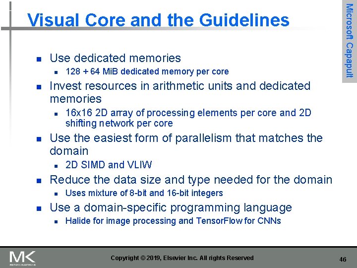
n Use dedicated memories n n Invest resources in arithmetic units and dedicated memories n n 2 D SIMD and VLIW Reduce the data size and type needed for the domain n n 16 x 16 2 D array of processing elements per core and 2 D shifting network per core Use the easiest form of parallelism that matches the domain n n 128 + 64 Mi. B dedicated memory per core Microsoft Capapult Visual Core and the Guidelines Uses mixture of 8 -bit and 16 -bit integers Use a domain-specific programming language n Halide for image processing and Tensor. Flow for CNNs Copyright © 2019, Elsevier Inc. All rights Reserved 46

Fallacy. It costs $100 million to design a custom chip. [HP mean: use FPGA; use modest changes to existing design. IMO, too “soft ideas” to call it a fallacy] Microsoft Capapult Fallacies and Pitfalls Pitfall. Performance counters added as an afterthought Fallacy. Architects are tackling the right DNN tasks [comment on too narrow focus of ISCA’ 16 DNN papers] Fallacy. For DNN hardware, inferences per second (IPS) is a fair summary performance metric [comparison should be among DNNs solving the same problem] Pitfall. Being ignorant of architecture history when designing an DSA [past computer architecture work that did not make it for general-purpose CPUs can become useful for DSAs. Example: systolic arrays] Copyright © 2019, Elsevier Inc. All rights Reserved 47