CIS 519419 Applied Machine Learning www seas upenn

CIS 519/419 Applied Machine Learning www. seas. upenn. edu/~cis 519 Dan Roth danroth@seas. upenn. edu http: //www. cis. upenn. edu/~danroth/ 461 C, 3401 Walnut Slides were created by Dan Roth (for CIS 519/419 at Penn or CS 446 at UIUC), Eric Eaton for CIS 519/419 at Penn, or from other authors who have made their ML slides available. CIS 419/519 Spring ’ 18

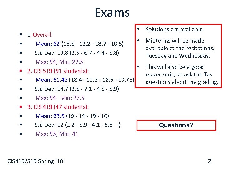
Exams • Solutions are available. § 1. Overall: • Midterms will be made § Mean: 62 (18. 6 - 13. 2 - 18. 7 - 10. 5) available at the recitations, § Std Dev: 13. 8 (2. 5 - 6. 7 - 4. 4 - 5. 8) Tuesday and Wednesday. § Max: 94, Min: 27. 5 • This will also be a good § 2. CIS 519 (91 students): opportunity to ask the Tas § Mean: 61. 48 (18. 4 - 12. 8 - 18. 5 - 10. 75) questions about the grading. § Std Dev: 14. 7 (2. 6 - 7. 1 - 4. 5 - 5. 9) § Max: 94 Min: 27. 5 § 3. CIS 419 (47 students): § Mean: 63. 6 (19 - 14 - 19 - 10) § Std Dev: 12 (2. 2 - 5. 9 - 4. 1 - 5. 8 ) Questions? § Max: 93, Min: 41 CIS 419/519 Spring ’ 18 2

Projects § Please start working! § Come to my office hours at least once in the next 3 weeks to discuss the project. CIS 419/519 Spring ’ 18 3

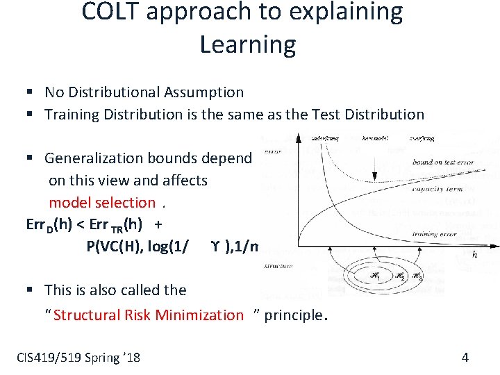
COLT approach to explaining Learning § No Distributional Assumption § Training Distribution is the same as the Test Distribution § Generalization bounds depend on this view and affects model selection. Err D(h) < Err TR (h) + P(VC(H), log(1/ ϒ ), 1/m) § This is also called the “ Structural Risk Minimization ” principle. CIS 419/519 Spring ’ 18 4

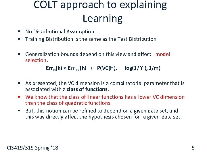
COLT approach to explaining Learning § No Distributional Assumption § Training Distribution is the same as the Test Distribution § Generalization bounds depend on this view and affect model selection. Err D(h) < Err TR (h) + P(VC(H), log(1/ ϒ ), 1/m) § As presented, the VC dimension is a combinatorial parameter that is associated with a class of functions. § We know that the class of linear functions has a lower VC dimension than the class of quadratic functions. § But, this notion can be refined to depend on a given data set, and this way directly affect the hypothesis chosen for a given data set. CIS 419/519 Spring ’ 18 5

Data Dependent VC dimension § So far we discussed VC dimension in the context of a fixed class of functions. § We can also parameterize the class of functions in interesting ways. § Consider the class of linear functions, parameterized by their margin. Note that this is a data dependent notion. CIS 419/519 Spring ’ 18 6

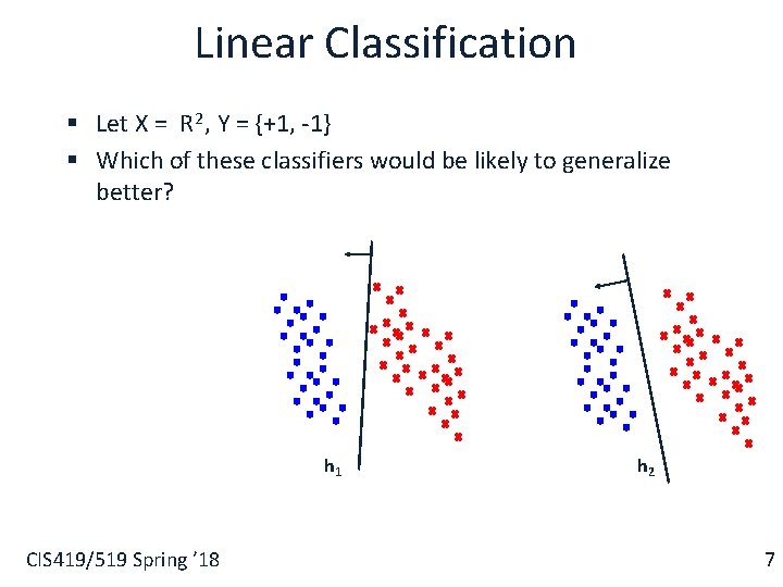
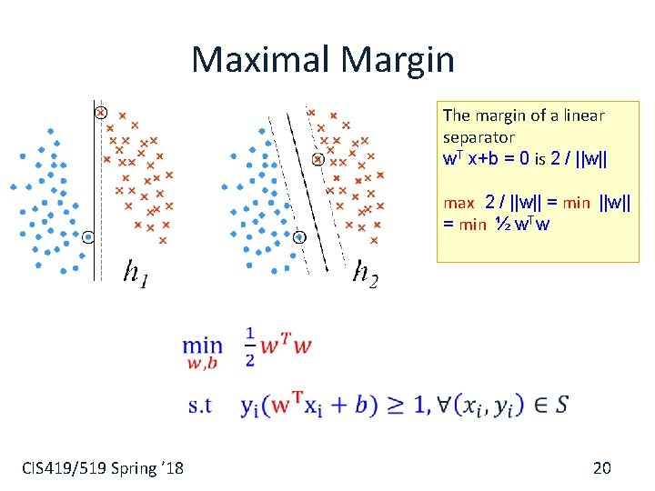
Linear Classification § Let X = R 2 , Y = {+1, -1} § Which of these classifiers would be likely to generalize better? h 1 CIS 419/519 Spring ’ 18 h 2 7

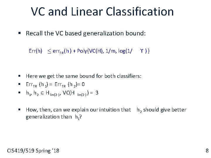
VC and Linear Classification § Recall the VC based generalization bound: Err(h) · err. TR (h ) + Poly{VC(H), 1/m, log(1/ ϒ )} § Here we get the same bound for both classifiers: § Err TR (h 1) = Err TR (h 2 )= 0 § h 1, h 2 2 H lin(2 ) , VC(H lin(2 ) ) = 3 § How, then, can we explain our intuition that h 2 should give better generalization than h 1? CIS 419/519 Spring ’ 18 8

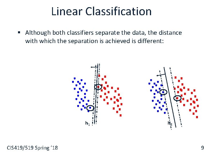
Linear Classification § Although both classifiers separate the data, the distance with which the separation is achieved is different: h 1 CIS 419/519 Spring ’ 18 h 2 9

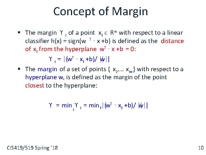
Concept of Margin § The margin ϒ i of a point xi Є R n with respect to a linear classifier h(x) = sign(w T ∙ x +b) is defined as the distance of xi from the hyperplane w. T ∙ x +b = 0: ϒ i = |(w. T ∙ xi +b)/ || w||| § The margin of a set of points { x 1, … xm } with respect to a hyperplane w, is defined as the margin of the point closest to the hyperplane: ϒ = min iϒ i = min i|(w. T ∙ xi +b)/ || w||| CIS 419/519 Spring ’ 18 10

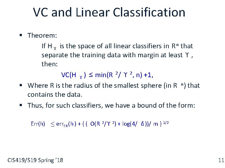
VC and Linear Classification § Theorem: If H ϒ is the space of all linear classifiers in R n that separate the training data with margin at least ϒ , then: VC(H ϒ ) ≤ min(R 2 / ϒ 2 , n) +1, § Where R is the radius of the smallest sphere (in R n) that contains the data. § Thus, for such classifiers, we have a bound of the form: Err(h) · err. TR (h ) + { ( O(R 2 /ϒ 2 ) + log(4/ δ))/ m } 1/2 CIS 419/519 Spring ’ 18 11

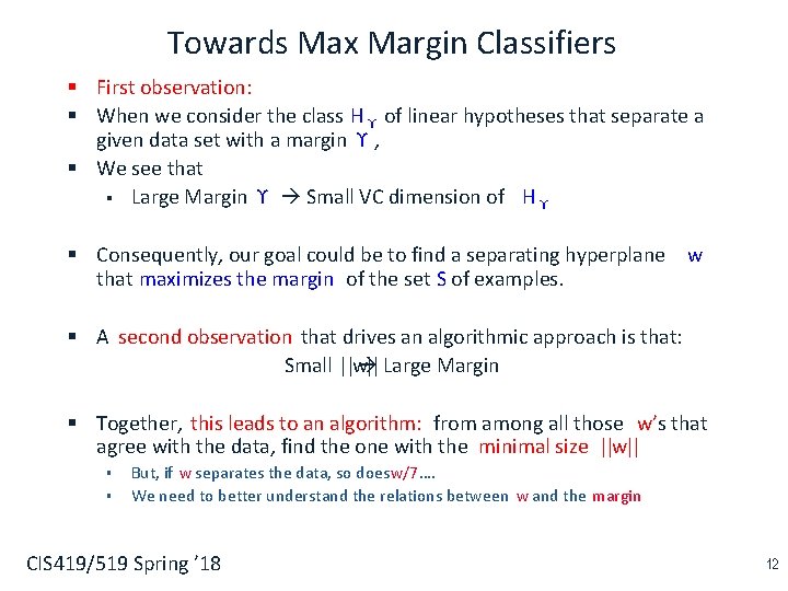
Towards Max Margin Classifiers § First observation: § When we consider the class H ϒ of linear hypotheses that separate a given data set with a margin ϒ , § We see that § Large Margin ϒ Small VC dimension of H ϒ § Consequently, our goal could be to find a separating hyperplane w that maximizes the margin of the set S of examples. § A second observation that drives an algorithmic approach is that: Small ||w|| Large Margin § Together, this leads to an algorithm: from among all those w’s that agree with the data, find the one with the minimal size ||w|| § § But, if w separates the data, so doesw/7…. We need to better understand the relations between w and the margin CIS 419/519 Spring ’ 18 12

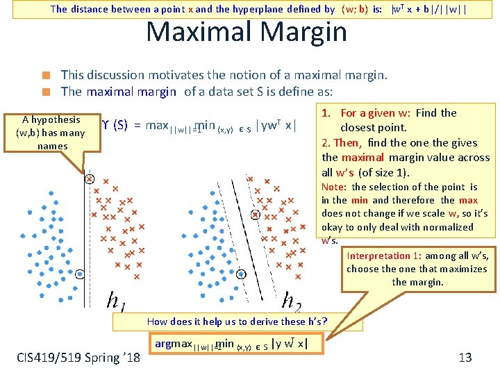
The distance between a point x and the hyperplane defined by ( w; b) is: |w. T x + b|/||w|| Maximal Margin This discussion motivates the notion of a maximal margin. The maximal margin of a data set S is define as: A hypothesis (w, b) has many names ϒ (S) = max ||w||=1 min (x, y) Є S |y w. T x| 1. For a given w: Find the closest point. 2. Then, find the one the gives the maximal margin value across all w’s (of size 1). Note: the selection of the point is in the min and therefore the max does not change if we scale w, so it’s okay to only deal with normalized w’s. Interpretation 1: among all w’s, choose the one that maximizes the margin. How does it help us to derive these h’s? CIS 419/519 Spring ’ 18 argmax ||w||=1 min (x, y) Є S |y w. T x| 13

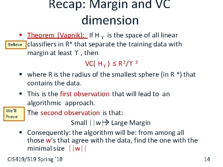
Recap: Margin and VC dimension § Theorem (Vapnik): If H ϒ is the space of all linear Believe classifiers in R n that separate the training data with margin at least ϒ , then VC( H ϒ ) ≤ R 2 /ϒ 2 § where R is the radius of the smallest sphere (in R n) that contains the data. § This is the first observation that will lead to an algorithmic approach. We’ll § The second observation is that: Prove Small ||w|| Large Margin § Consequently: the algorithm will be: from among all those w’s that agree with the data, find the one with the minimal size ||w|| CIS 419/519 Spring ’ 18 14

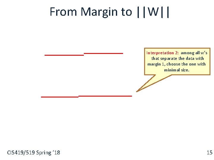
From Margin to ||W|| § Interpretation 2: among all w’s that separate the data with margin 1, choose the one with minimal size. CIS 419/519 Spring ’ 18 15

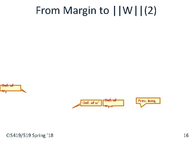
From Margin to ||W||(2) § Def. of w 0 Def. of w’ CIS 419/519 Spring ’ 18 Def. of w 0 Prev. ineq. 16

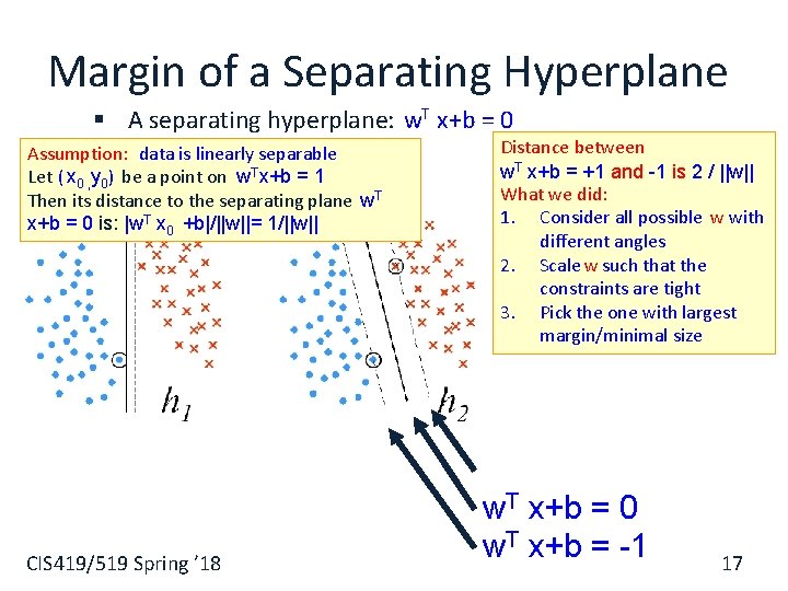
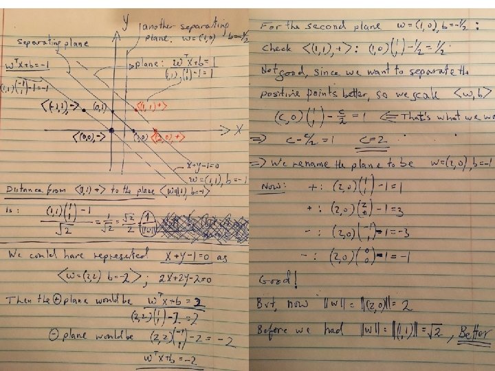
Margin of a Separating Hyperplane § A separating hyperplane: w. T x+b = 0 Assumption: data is linearly separable Let ( x 0 , y 0) be a point on w. Tx+b = 1 Then its distance to the separating plane w. T x+b = 0 is: |w. T x 0 +b|/||w||= 1/||w|| CIS 419/519 Spring ’ 18 Distance between w. T x+b = +1 and -1 is 2 / ||w|| What we did: 1. Consider all possible w with different angles 2. Scale w such that the constraints are tight 3. Pick the one with largest margin/minimal size w. T x+b = 0 w. T x+b = -1 17

CIS 419/519 Spring ’ 18 18

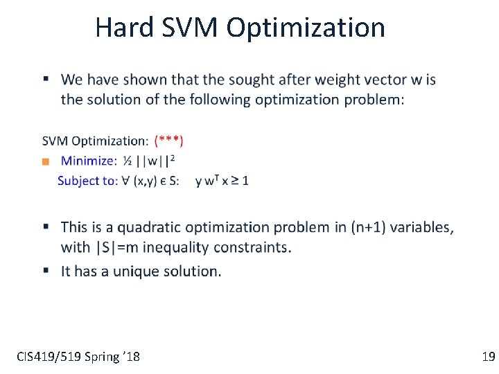
Hard SVM Optimization § CIS 419/519 Spring ’ 18 19

Maximal Margin The margin of a linear separator w. T x+b = 0 is 2 / ||w|| max 2 / ||w|| = min ½ w. Tw CIS 419/519 Spring ’ 18 20

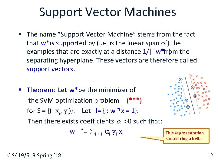
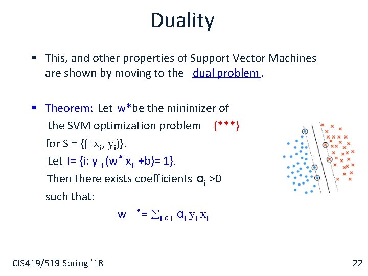
Support Vector Machines § The name “Support Vector Machine” stems from the fact that w*is supported by (i. e. is the linear span of) the examples that are exactly at a distance 1/||w*|| from the separating hyperplane. These vectors are therefore called support vectors. § Theorem: Let w*be the minimizer of the SVM optimization problem (***) for S = {( xi, yi)}. Let I= {i: w *T x = 1}. Then there exists coefficients ®i >0 such that: w * = i Є I αi yi xi CIS 419/519 Spring ’ 18 This representation should ring a bell… 21

Duality § This, and other properties of Support Vector Machines are shown by moving to the dual problem. § Theorem: Let w*be the minimizer of the SVM optimization problem (***) for S = {( xi, yi)}. Let I= {i: y i (w *T xi +b)= 1}. Then there exists coefficients αi >0 such that: w * = i Є I αi yi xi CIS 419/519 Spring ’ 18 22

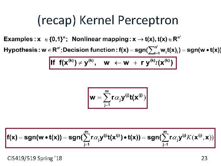
(recap) Kernel Perceptron § CIS 419/519 Spring ’ 18 23

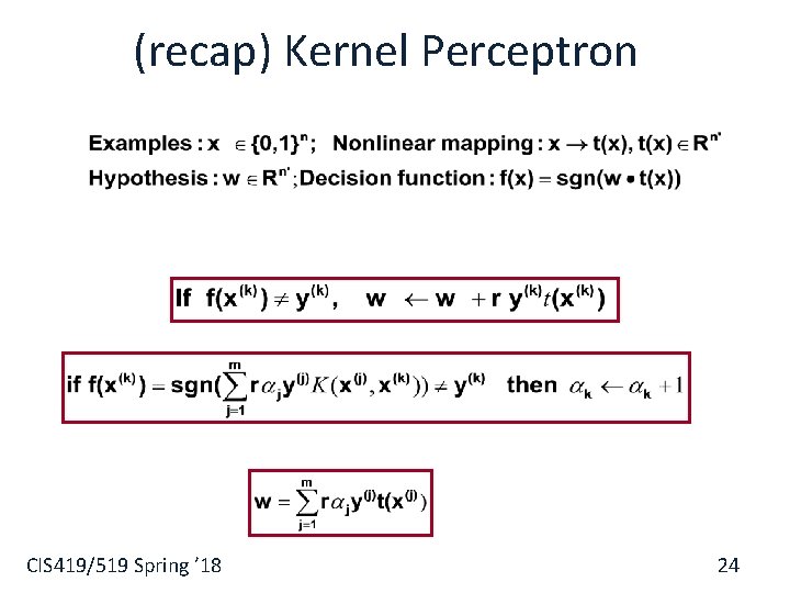
(recap) Kernel Perceptron § CIS 419/519 Spring ’ 18 24

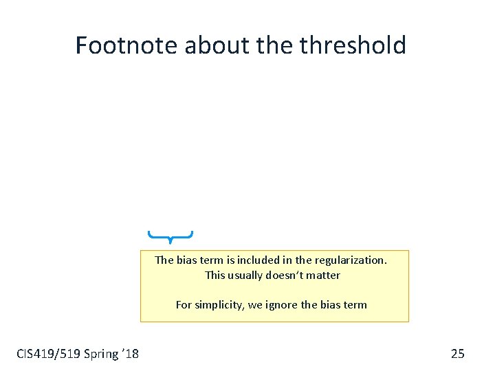
Footnote about the threshold § The bias term is included in the regularization. This usually doesn’t matter For simplicity, we ignore the bias term CIS 419/519 Spring ’ 18 25

Key Issues § Computational Issues § § Training of an SVM used to be is very time consuming – solving quadratic program. Modern methods are based on Stochastic Gradient Descent and Coordinate Descent and are much faster. § Is it really optimal? § Is the objective function we are optimizing the “right” one? CIS 419/519 Spring ’ 18 26

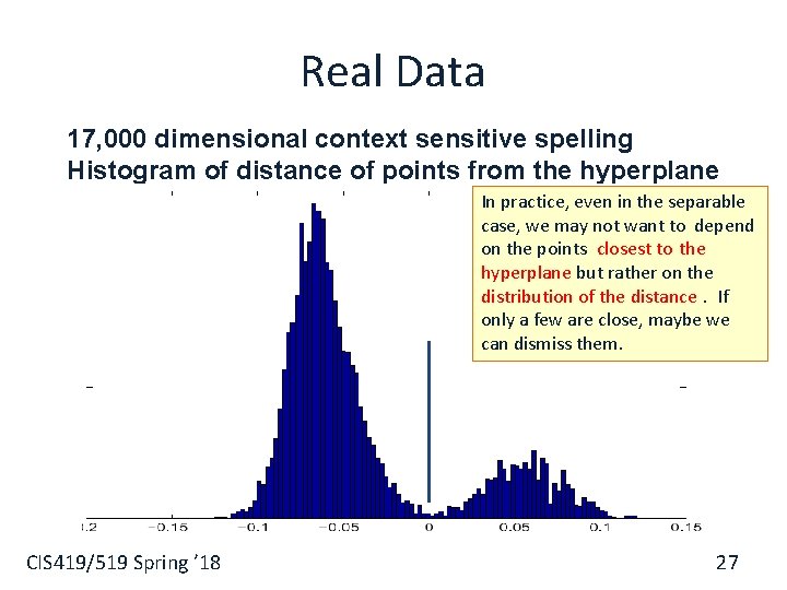
Real Data 17, 000 dimensional context sensitive spelling Histogram of distance of points from the hyperplane In practice, even in the separable case, we may not want to depend on the points closest to the hyperplane but rather on the distribution of the distance. If only a few are close, maybe we can dismiss them. CIS 419/519 Spring ’ 18 27

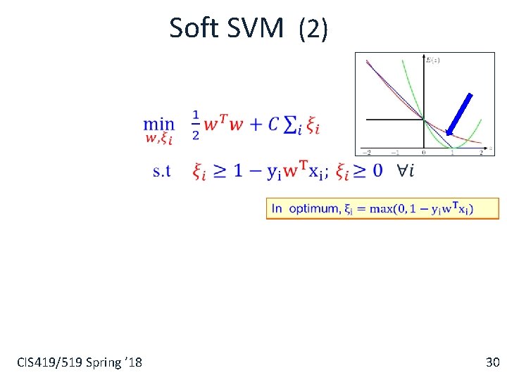
Soft SVM § The hard SVM formulation assumes linearly separable data. § A natural relaxation: § maximize the margin while minimizing the # of examples that violate the margin (separability) constraints. § However, this leads to non-convex problem that is hard to solve. § Instead, we relax in a different way, that results in optimizing a surrogate loss function that is convex. CIS 419/519 Spring ’ 18 28

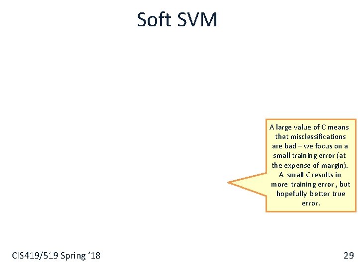
Soft SVM § A large value of C means that misclassifications are bad – we focus on a small training error (at the expense of margin). A small C results in more training error , but hopefully better true error. CIS 419/519 Spring ’ 18 29

Soft SVM (2) § CIS 419/519 Spring ’ 18 30

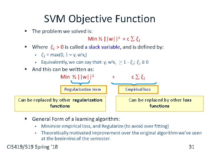
SVM Objective Function § Regularization term Can be replaced by other regularization functions CIS 419/519 Spring ’ 18 Empirical loss Can be replaced by other loss functions 31

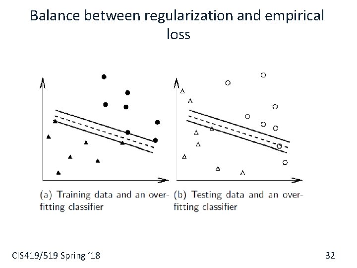
Balance between regularization and empirical loss CIS 419/519 Spring ’ 18 32

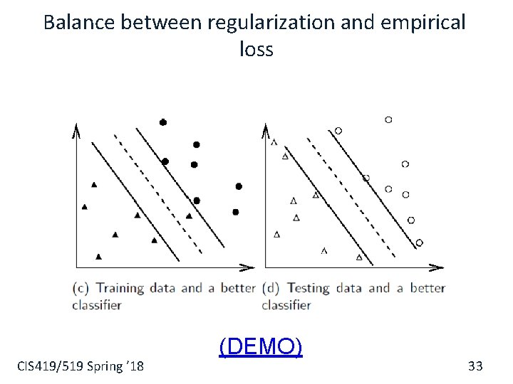
Balance between regularization and empirical loss CIS 419/519 Spring ’ 18 (DEMO) 33

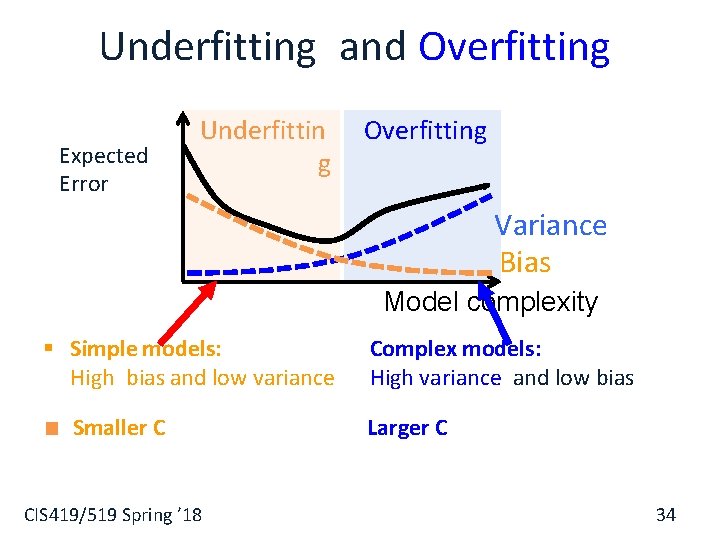
Underfitting and Overfitting Expected Error Underfittin g Overfitting Variance Bias Model complexity § Simple models: High bias and low variance Smaller C CIS 419/519 Spring ’ 18 Complex models: High variance and low bias Larger C 34

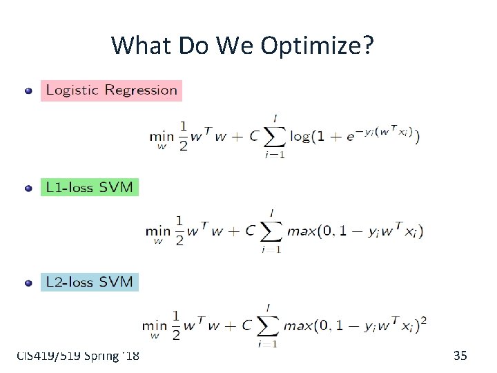
What Do We Optimize? CIS 419/519 Spring ’ 18 35

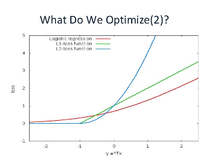
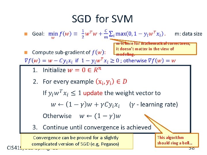
What Do We Optimize(2)? § We get an unconstrained problem. We can use the gradient descent algorithm ! However, it is quite slow. § Many other methods § § Iterative scaling; non-linear conjugate gradient; quasi-Newton methods; truncated Newton methods; trust-region newton method. All methods are iterative methods, that generate a sequence wk that converges to the optimal solution of the optimization problem above. § Currently: Limited memory BFGS is very popular CIS 419/519 Spring ’ 18 36

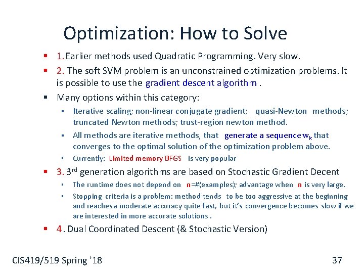
Optimization: How to Solve § 1. Earlier methods used Quadratic Programming. Very slow. § 2. The soft SVM problem is an unconstrained optimization problems. It is possible to use the gradient descent algorithm. § Many options within this category: § § § Iterative scaling; non-linear conjugate gradient; quasi-Newton methods; truncated Newton methods; trust-region newton method. All methods are iterative methods, that generate a sequence wk that converges to the optimal solution of the optimization problem above. Currently: Limited memory BFGS is very popular § 3. 3 rd generation algorithms are based on Stochastic Gradient Decent § § The runtime does not depend on n=#(examples); advantage when n is very large. Stopping criteria is a problem: method tends to be too aggressive at the beginning and reaches a moderate accuracy quite fast, but it’s convergence becomes slow if we are interested in more accurate solutions. § 4. Dual Coordinated Descent (& Stochastic Version) CIS 419/519 Spring ’ 18 37

SGD for SVM § m is here for mathematical correctness, it doesn’t matter in the view of modeling. Convergence can be proved for a slightly complicated version of SGD (e. g, Pegasos) CIS 419/519 Spring ’ 18 This algorithm should ring a bell… 38

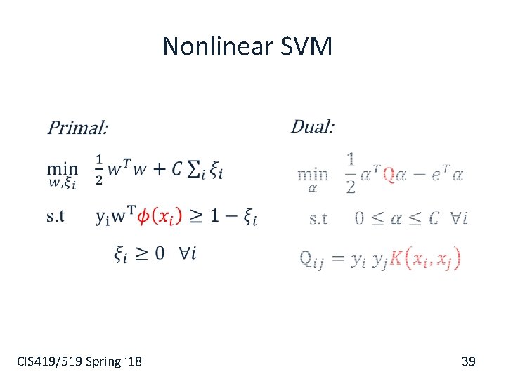
Nonlinear SVM § CIS 419/519 Spring ’ 18 39

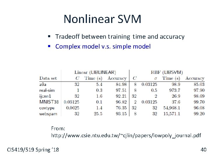
Nonlinear SVM § Tradeoff between training time and accuracy § Complex model v. s. simple model From: http: //www. csie. ntu. edu. tw/~cjlin/papers/lowpoly_journal. pdf CIS 419/519 Spring ’ 18 40