CIS 519419 Applied Machine Learning www seas upenn

CIS 519/419 Applied Machine Learning www. seas. upenn. edu/~cis 519 Dan Roth danroth@seas. upenn. edu http: //www. cis. upenn. edu/~danroth/ 461 C, 3401 Walnut Slides were created by Dan Roth (for CIS 519/419 at Penn or CS 446 at UIUC), Eric Eaton for CIS 519/419 at Penn, or from other authors who have made their ML slides available. CIS 419/519 Fall ’ 19

Administration § Midterm Exam next Wednesday 10/31 § In class Questions § Closed books § Examples are on the web site § All the material covered in class and HW § Go to the recitation § HW 2 is due on Wednesday week 10/24 § § Check Piazza posts about efficiency Go to office hours CIS 419/519 Fall ’ 19 2

Projects https: //www. seas. upenn. edu/~cis 519/fall 2018/project. html § CIS 519 students need to do a team project § Teams will be of size 2 -3 § Projects proposals are due on Friday 10/26/18 § § § Details will be available on the website We will give comments and/or requests to modify / augment/ do a different project. There may also be a mechanism for peer comments. § Please start thinking and working on the project now. § Your proposal is limited to 1 -2 pages, but needs to include references and, ideally, some preliminary results/ideas. § Any project with a significant Machine Learning component is good. § § § Experimental work, theoretical work, a combination of both or a critical survey of results in some specialized topic. The work has to include some reading of the literature. Originality is not mandatory but is encouraged. § Try to make it interesting! CIS 419/519 Fall ’ 19 3

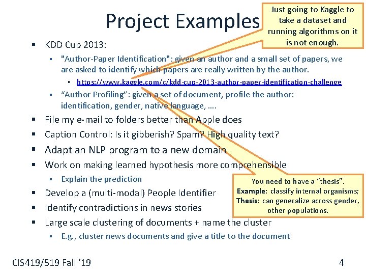
Project Examples § KDD Cup 2013: § "Author-Paper Identification": given an author and a small set of papers, we are asked to identify which papers are really written by the author. § § Just going to Kaggle to take a dataset and running algorithms on it is not enough. https: //www. kaggle. com/c/kdd-cup-2013 -author-paper-identification-challenge “Author Profiling”: given a set of document, profile the author: identification, gender, native language, …. § File my e-mail to folders better than Apple does § Caption Control: Is it gibberish? Spam? High quality text? § Adapt an NLP program to a new domain § Work on making learned hypothesis more comprehensible § Explain the prediction You need to have a “thesis”. Example: classify internal organisms; Thesis: can generalize across gender, other populations. § Develop a (multi-modal) People Identifier § Identify contradictions in news stories § Large scale clustering of documents + name the cluster § E. g. , cluster news documents and give a title to the document CIS 419/519 Fall ’ 19 4

Where are we? § Algorithmically: § § Perceptron + Variations (Stochastic) Gradient Descent § Models: § Online Learning; Mistake Driven Learning § What do we know about Generalization? (to previously unseen examples? ) § How will your algorithm do on the next example? § Next we develop a theory of Generalization. § We will come back to the same (or very similar) algorithms and show the new theory sheds light on appropriate modifications of them, and provides guarantees. CIS 419/519 Fall ’ 19 5

Computational Learning Theory § What general laws constrain inductive learning ? § § What learning problems can be solved ? When can we trust the output of a learning algorithm ? § We seek theory to relate § § § Probability of successful Learning Number of training examples Complexity of hypothesis space Accuracy to which target concept is approximated Manner in which training examples are presented CIS 419/519 Fall ’ 19 6

Recall what we did earlier: Quantifying Performance § We want to be able to say something rigorous about the performance of our learning algorithm. § We will concentrate on discussing the number of examples one needs to see before we can say that our learned hypothesis is good. CIS 419/519 Fall ’ 19 7

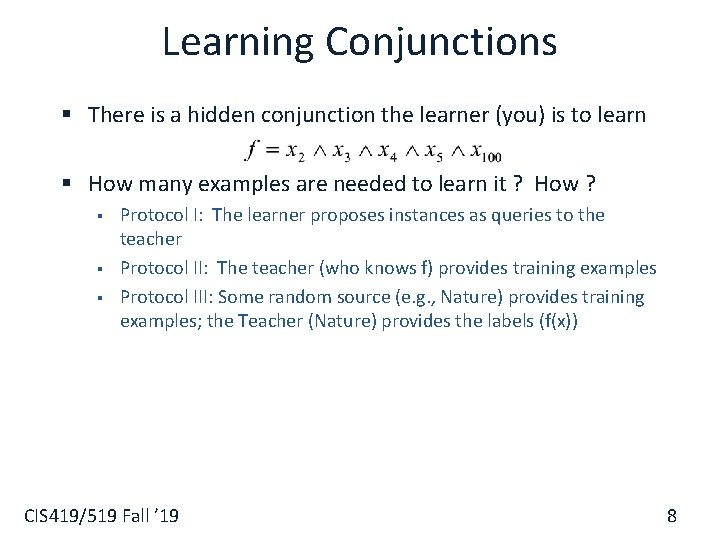
Learning Conjunctions § There is a hidden conjunction the learner (you) is to learn § How many examples are needed to learn it ? How ? § § § Protocol I: The learner proposes instances as queries to the teacher Protocol II: The teacher (who knows f) provides training examples Protocol III: Some random source (e. g. , Nature) provides training examples; the Teacher (Nature) provides the labels (f(x)) CIS 419/519 Fall ’ 19 8

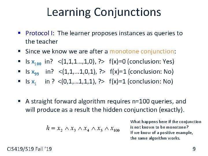
Learning Conjunctions § Protocol I: The learner proposes instances as queries to the teacher § Since we know we are after a monotone conjunction: § Is x 100 in? <(1, 1, 1…, 1, 0), ? > f(x)=0 (conclusion: Yes) § Is x 99 in? <(1, 1, … 1, 0, 1), ? > f(x)=1 (conclusion: No) § Is x 1 in ? <(0, 1, … 1, 1, 1), ? > f(x)=1 (conclusion: No) § A straight forward algorithm requires n=100 queries, and will produce as a result the hidden conjunction (exactly). What happens here if the conjunction is not known to be monotone? If we know of a positive example, the same algorithm works. CIS 419/519 Fall ’ 19 9

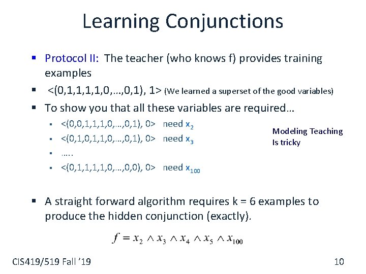
Learning Conjunctions § Protocol II: The teacher (who knows f) provides training examples § <(0, 1, 1, 0, …, 0, 1), 1> (We learned a superset of the good variables) § To show you that all these variables are required… § § <(0, 0, 1, 1, 1, 0, …, 0, 1), 0> need x 2 <(0, 1, 1, 0, …, 0, 1), 0> need x 3 …. . <(0, 1, 1, 0, …, 0, 0), 0> need x 100 Modeling Teaching Is tricky § A straight forward algorithm requires k = 6 examples to produce the hidden conjunction (exactly). CIS 419/519 Fall ’ 19 10

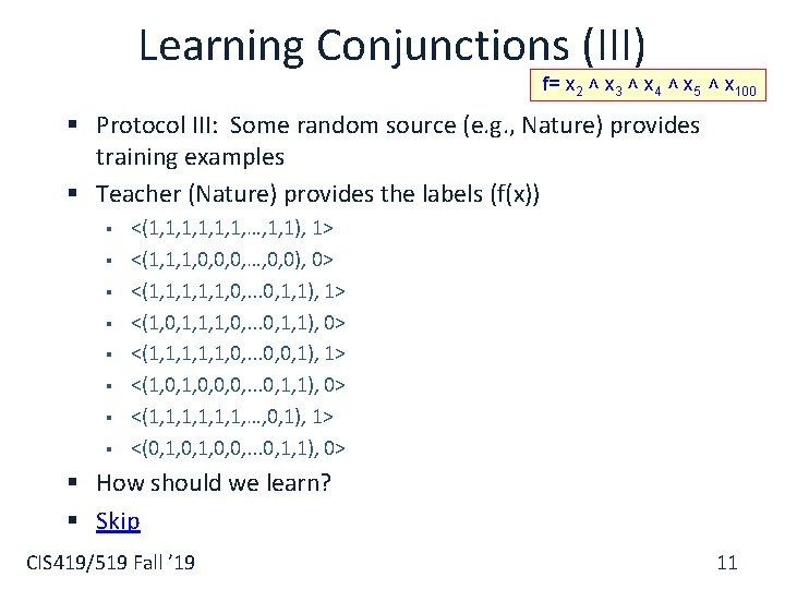
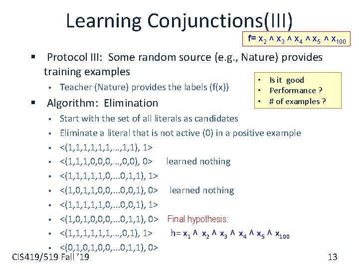
Learning Conjunctions (III) f= x 2 ˄ x 3 ˄ x 4 ˄ x 5 ˄ x 100 § Protocol III: Some random source (e. g. , Nature) provides training examples § Teacher (Nature) provides the labels (f(x)) § § § § <(1, 1, 1, …, 1, 1), 1> <(1, 1, 1, 0, 0, 0, …, 0, 0), 0> <(1, 1, 1, 0, . . . 0, 1, 1), 1> <(1, 0, 1, 1, 1, 0, . . . 0, 1, 1), 0> <(1, 1, 1, 0, . . . 0, 0, 1), 1> <(1, 0, 0, 0, . . . 0, 1, 1), 0> <(1, 1, 1, …, 0, 1), 1> <(0, 1, 0, 0, . . . 0, 1, 1), 0> § How should we learn? § Skip CIS 419/519 Fall ’ 19 11

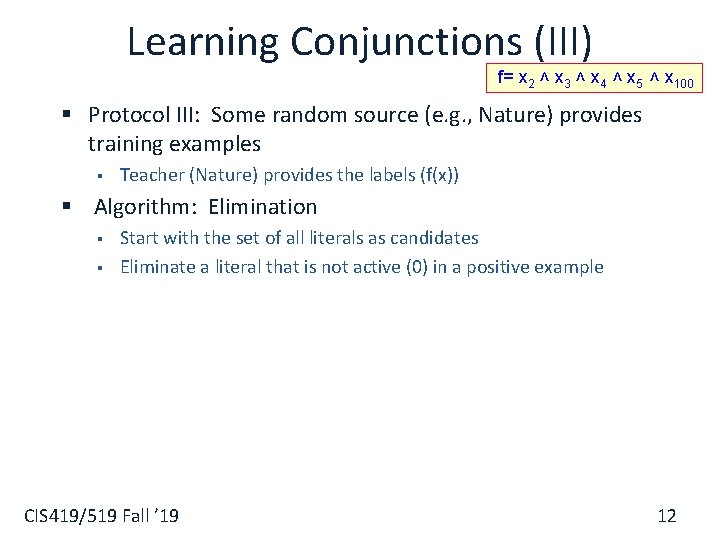
Learning Conjunctions (III) f= x 2 ˄ x 3 ˄ x 4 ˄ x 5 ˄ x 100 § Protocol III: Some random source (e. g. , Nature) provides training examples § Teacher (Nature) provides the labels (f(x)) § Algorithm: Elimination § § Start with the set of all literals as candidates Eliminate a literal that is not active (0) in a positive example CIS 419/519 Fall ’ 19 12

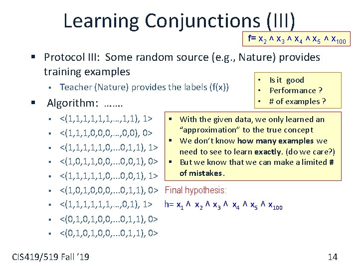
Learning Conjunctions(III) f= x 2 ˄ x 3 ˄ x 4 ˄ x 5 ˄ x 100 § Protocol III: Some random source (e. g. , Nature) provides training examples § Teacher (Nature) provides the labels (f(x)) § Algorithm: Elimination • Is it good • Performance ? • # of examples ? Start with the set of all literals as candidates § Eliminate a literal that is not active (0) in a positive example § <(1, 1, 1, …, 1, 1), 1> § <(1, 1, 1, 0, 0, 0, …, 0, 0), 0> learned nothing § <(1, 1, 1, 0, . . . 0, 1, 1), 1> § <(1, 0, 1, 1, 0, 0, . . . 0, 0, 1), 0> learned nothing § <(1, 1, 1, 0, . . . 0, 0, 1), 1> § <(1, 0, 0, 0, . . . 0, 1, 1), 0> Final hypothesis: § <(1, 1, 1, …, 0, 1), 1> h= x 1 ˄ x 2 ˄ x 3 ˄ x 4 ˄ x 5 ˄ x 100 § <(0, 1, 0, 0, . . . 0, 1, 1), 0> CIS 419/519 Fall ’ 19 § 13

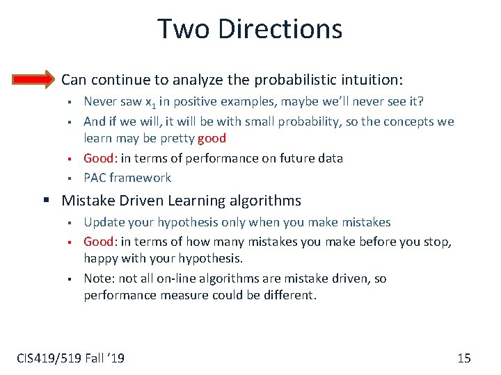
Learning Conjunctions (III) f= x 2 ˄ x 3 ˄ x 4 ˄ x 5 ˄ x 100 § Protocol III: Some random source (e. g. , Nature) provides training examples § Teacher (Nature) provides the labels (f(x)) § Algorithm: ……. § § § § § • Is it good • Performance ? • # of examples ? <(1, 1, 1, …, 1, 1), 1> § With the given data, we only learned an <(1, 1, 1, 0, 0, 0, …, 0, 0), 0> “approximation” to the true concept § We don’t know how many examples we <(1, 1, 1, 0, . . . 0, 1, 1), 1> need to see to learn exactly. (do we care? ) <(1, 0, 1, 1, 0, 0, . . . 0, 0, 1), 0> § But we know that we can make a limited # of mistakes. <(1, 1, 1, 0, . . . 0, 0, 1), 1> <(1, 0, 0, 0, . . . 0, 1, 1), 0> Final hypothesis: <(1, 1, 1, …, 0, 1), 1> h= x 1 ˄ x 2 ˄ x 3 ˄ x 4 ˄ x 5 ˄ x 100 <(0, 1, 0, 0, . . . 0, 1, 1), 0> CIS 419/519 Fall ’ 19 14

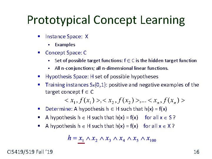
Two Directions § Can continue to analyze the probabilistic intuition: § § Never saw x 1 in positive examples, maybe we’ll never see it? And if we will, it will be with small probability, so the concepts we learn may be pretty good Good: in terms of performance on future data PAC framework § Mistake Driven Learning algorithms § § § Update your hypothesis only when you make mistakes Good: in terms of how many mistakes you make before you stop, happy with your hypothesis. Note: not all on-line algorithms are mistake driven, so performance measure could be different. CIS 419/519 Fall ’ 19 15

Prototypical Concept Learning § Instance Space: X § Examples § Concept Space: C § § Set of possible target functions: f 2 C is the hidden target function All n-conjunctions; all n-dimensional linear functions. § Hypothesis Space: H set of possible hypotheses § Training instances Sx{0, 1}: positive and negative examples of the target concept f C § Determine: A hypothesis h H such that h(x) = f(x) § A hypothesis h H such that h(x) = f(x) for all x S ? § A hypothesis h H such that h(x) = f(x) for all x X ? CIS 419/519 Fall ’ 19 16

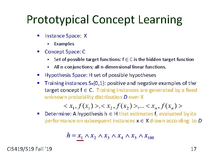
Prototypical Concept Learning § Instance Space: X § Examples § Concept Space: C § § Set of possible target functions: f 2 C is the hidden target function All n-conjunctions; all n-dimensional linear functions. § Hypothesis Space: H set of possible hypotheses § Training instances Sx{0, 1}: positive and negative examples of the target concept f C. Training instances are generated by a fixed unknown probability distribution D over X § Determine: A hypothesis h H that estimates f, evaluated by its performance on subsequent instances x X drawn according to D CIS 419/519 Fall ’ 19 17

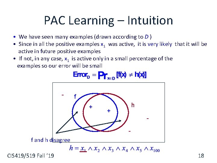
PAC Learning – Intuition • We have seen many examples (drawn according to D ) • Since in all the positive examples x 1 was active, it is very likely that it will be active in future positive examples • If not, in any case, x 1 is active only in a small percentage of the examples so our error will be small - f + h + f and h disagree CIS 419/519 Fall ’ 19 18

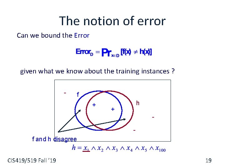
The notion of error Can we bound the Error given what we know about the training instances ? - f + h + f and h disagree CIS 419/519 Fall ’ 19 19

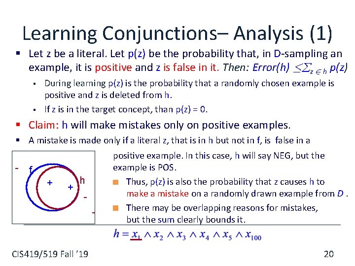
Learning Conjunctions– Analysis (1) § Let z be a literal. Let p(z) be the probability that, in D-sampling an example, it is positive and z is false in it. Then: Error(h) · z 2 h p(z) § § During learning p(z) is the probability that a randomly chosen example is positive and z is deleted from h. If z is in the target concept, than p(z) = 0. § Claim: h will make mistakes only on positive examples. § A mistake is made only if a literal z, that is in h but not in f, is false in a - f + + h - CIS 419/519 Fall ’ 19 positive example. In this case, h will say NEG, but the example is POS. Thus, p(z) is also the probability that z causes h to make a mistake on a randomly drawn example from D. There may be overlapping reasons for mistakes, but the sum clearly bounds it. 20

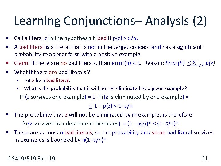
Learning Conjunctions– Analysis (2) § Call a literal z in the hypothesis h bad if p(z) > /n. § A bad literal is a literal that is not in the target concept and has a significant probability to appear false with a positive example. § Claim: If there are no bad literals, than error(h) < . Reason: Error(h) · z 2 h p(z) § What if there are bad literals ? § § Let z be a bad literal. What is the probability that it will not be eliminated by a given example? Pr(z survives one example) = 1 - Pr(z is eliminated by one example) = · 1 – p(z) < 1 - /n § The probability that z will not be eliminated by m examples is therefore: Pr(z survives m independent examples) = (1 –p(z))m < (1 - /n)m § There at most n bad literals, so the probability that some bad literal survives m examples is bounded by n(1 - /n)m CIS 419/519 Fall ’ 19 21

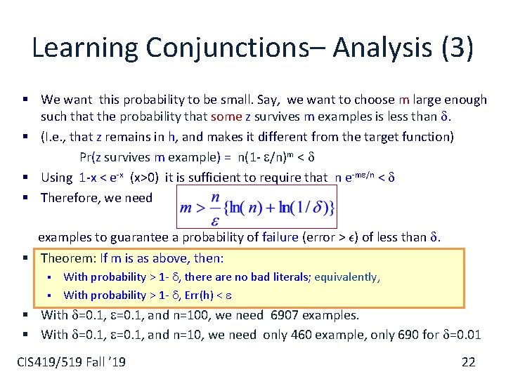
Learning Conjunctions– Analysis (3) § We want this probability to be small. Say, we want to choose m large enough such that the probability that some z survives m examples is less than . § (I. e. , that z remains in h, and makes it different from the target function) Pr(z survives m example) = n(1 - /n)m < § Using 1 -x < e-x (x>0) it is sufficient to require that n e-m /n < § Therefore, we need examples to guarantee a probability of failure (error > ²) of less than . § Theorem: If m is as above, then: § § With probability > 1 - , there are no bad literals; equivalently, With probability > 1 - , Err(h) < § With =0. 1, and n=100, we need 6907 examples. § With =0. 1, and n=10, we need only 460 example, only 690 for =0. 01 CIS 419/519 Fall ’ 19 22

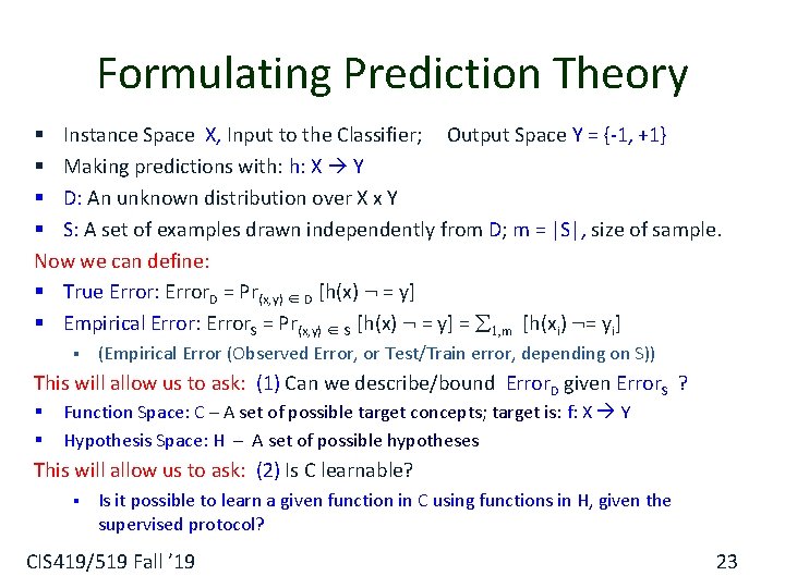
Formulating Prediction Theory § Instance Space X, Input to the Classifier; Output Space Y = {-1, +1} § Making predictions with: h: X Y § D: An unknown distribution over X x Y § S: A set of examples drawn independently from D; m = |S|, size of sample. Now we can define: § True Error: Error. D = Pr(x, y) ∈ D [h(x) : = y] § Empirical Error: Error. S = Pr(x, y) ∈ S [h(x) : = y] = 1, m [h(xi) : = yi] § (Empirical Error (Observed Error, or Test/Train error, depending on S)) This will allow us to ask: (1) Can we describe/bound Error. D given Error. S ? § § Function Space: C – A set of possible target concepts; target is: f: X Y Hypothesis Space: H – A set of possible hypotheses This will allow us to ask: (2) Is C learnable? § Is it possible to learn a given function in C using functions in H, given the supervised protocol? CIS 419/519 Fall ’ 19 23

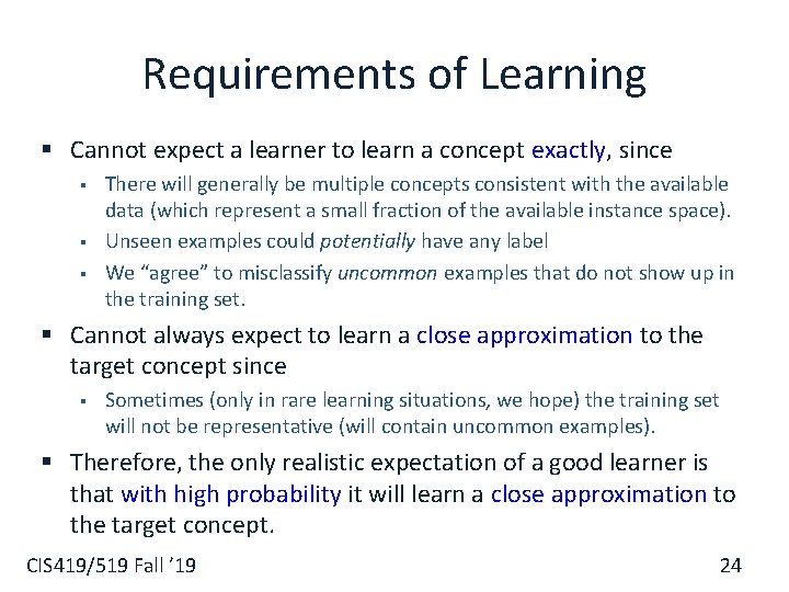
Requirements of Learning § Cannot expect a learner to learn a concept exactly, since § § § There will generally be multiple concepts consistent with the available data (which represent a small fraction of the available instance space). Unseen examples could potentially have any label We “agree” to misclassify uncommon examples that do not show up in the training set. § Cannot always expect to learn a close approximation to the target concept since § Sometimes (only in rare learning situations, we hope) the training set will not be representative (will contain uncommon examples). § Therefore, the only realistic expectation of a good learner is that with high probability it will learn a close approximation to the target concept. CIS 419/519 Fall ’ 19 24

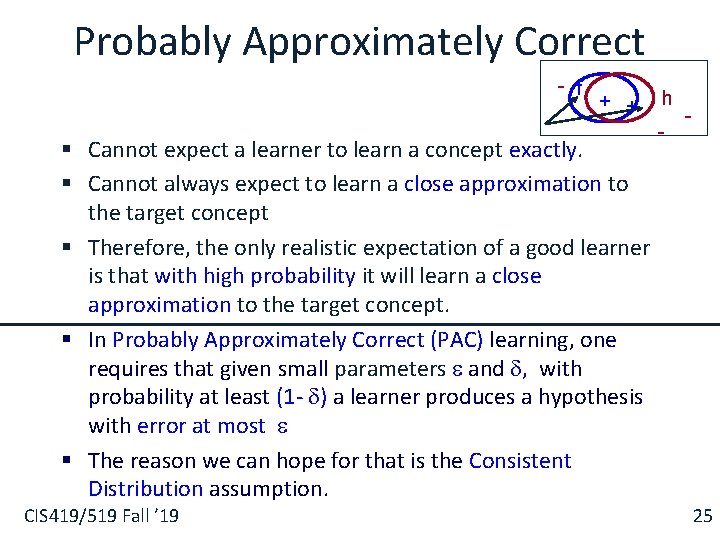
Probably Approximately Correct - f + + § Cannot expect a learner to learn a concept exactly. § Cannot always expect to learn a close approximation to the target concept § Therefore, the only realistic expectation of a good learner is that with high probability it will learn a close approximation to the target concept. § In Probably Approximately Correct (PAC) learning, one requires that given small parameters and , with probability at least (1 - ) a learner produces a hypothesis with error at most § The reason we can hope for that is the Consistent Distribution assumption. CIS 419/519 Fall ’ 19 h - - 25

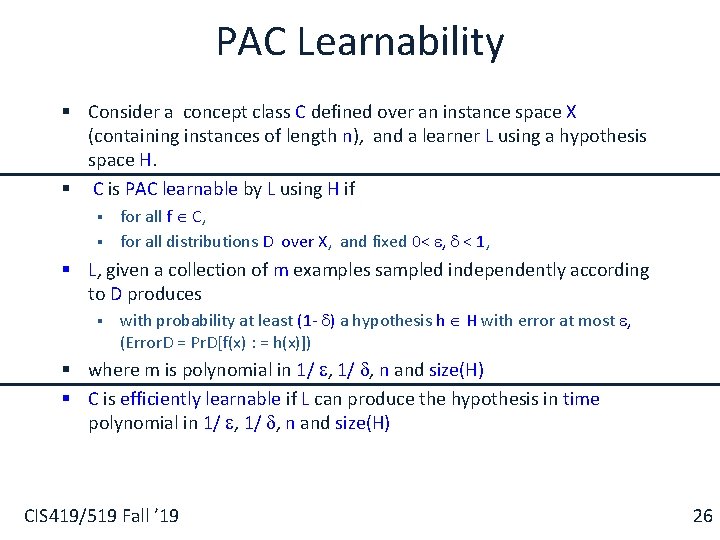
PAC Learnability § Consider a concept class C defined over an instance space X (containing instances of length n), and a learner L using a hypothesis space H. § C is PAC learnable by L using H if § § for all f C, for all distributions D over X, and fixed 0< , < 1, § L, given a collection of m examples sampled independently according to D produces § with probability at least (1 - ) a hypothesis h H with error at most , (Error. D = Pr. D[f(x) : = h(x)]) § where m is polynomial in 1/ , n and size(H) § C is efficiently learnable if L can produce the hypothesis in time polynomial in 1/ , n and size(H) CIS 419/519 Fall ’ 19 26

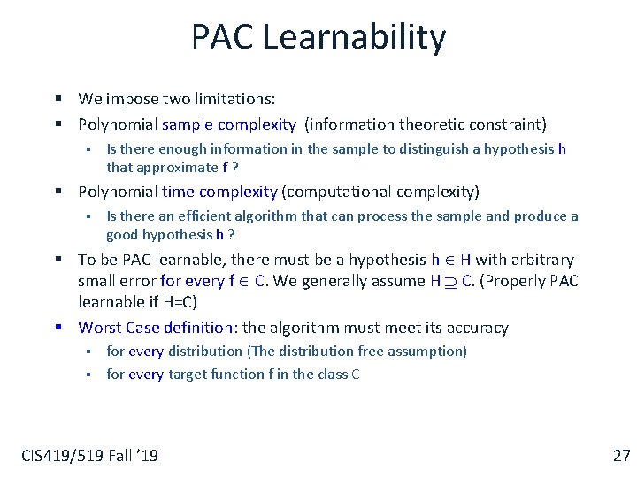
PAC Learnability § We impose two limitations: § Polynomial sample complexity (information theoretic constraint) § Is there enough information in the sample to distinguish a hypothesis h that approximate f ? § Polynomial time complexity (computational complexity) § Is there an efficient algorithm that can process the sample and produce a good hypothesis h ? § To be PAC learnable, there must be a hypothesis h H with arbitrary small error for every f C. We generally assume H C. (Properly PAC learnable if H=C) § Worst Case definition: the algorithm must meet its accuracy § § for every distribution (The distribution free assumption) for every target function f in the class C CIS 419/519 Fall ’ 19 27

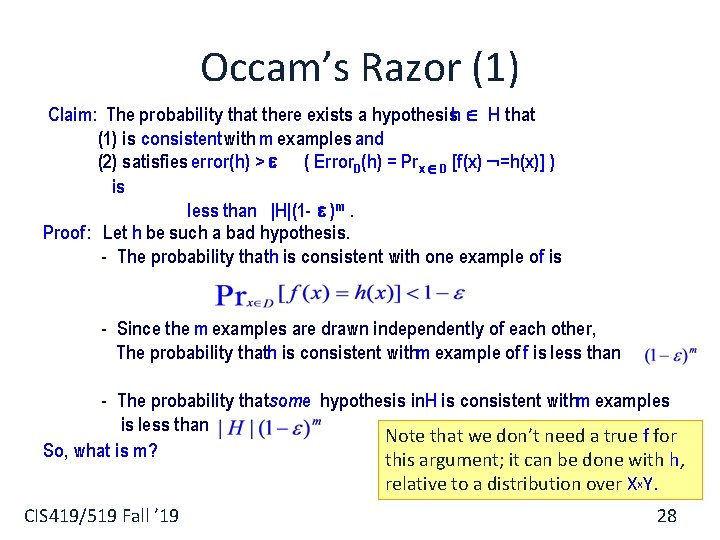
Occam’s Razor (1) Claim: The probability that there exists a hypothesish H that (1) is consistentwith m examples and (2) satisfies error(h) > ( Error. D(h) = Pr x 2 D [f(x) : =h(x)] ) is less than |H|(1 - )m. Proof: Let h be such a bad hypothesis. - The probability thath is consistent with one example off is - Since the m examples are drawn independently of each other, The probability thath is consistent withm example of f is less than - The probability thatsome hypothesis in. H is consistent withm examples is less than Note that we don’t need a true f for So, what is m? this argument; it can be done with h, relative to a distribution over Xx. Y. CIS 419/519 Fall ’ 19 28

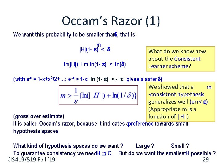
Occam’s Razor (1) We want this probability to be smaller than , that is: m |H|(1 - ) < ln(|H|) + m ln(1 - ) < ln( ) What do we know about the Consistent Learner scheme? (with e-x = 1 -x+x 2/2+…; e -x > 1 -x; ln (1 - ) < - ; gives a safer ) We showed that a m -consistent hypothesis generalizes well (err< ) (Appropriate m is a (gross over estimate) function of |H|) It is called Occam’s razor, because it indicates apreference towards small hypothesis spaces What kind of hypothesis spaces do we want ? Large ? Small ? To guarantee consistency we need. H C. But do we want the smallest. H possible ? 29 CIS 419/519 Fall ’ 19

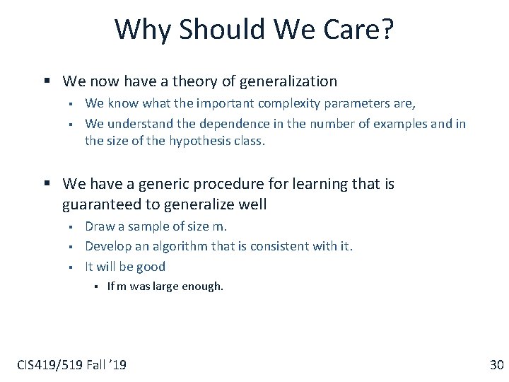
Why Should We Care? § We now have a theory of generalization § § We know what the important complexity parameters are, We understand the dependence in the number of examples and in the size of the hypothesis class. § We have a generic procedure for learning that is guaranteed to generalize well § § § Draw a sample of size m. Develop an algorithm that is consistent with it. It will be good § If m was large enough. CIS 419/519 Fall ’ 19 30

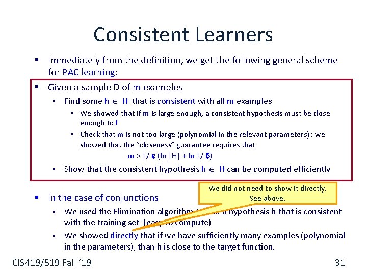
Consistent Learners § Immediately from the definition, we get the following general scheme for PAC learning: § Given a sample D of m examples § Find some h H that is consistent with all m examples We showed that if m is large enough, a consistent hypothesis must be close enough to f § Check that m is not too large (polynomial in the relevant parameters) : we showed that the “closeness” guarantee requires that m > 1/ (ln |H| + ln 1/ ) § § Show that the consistent hypothesis h H can be computed efficiently § In the case of conjunctions § § We did not need to show it directly. See above. We used the Elimination algorithm to find a hypothesis h that is consistent with the training set (easy to compute) We showed directly that if we have sufficiently many examples (polynomial in the parameters), than h is close to the target function. CIS 419/519 Fall ’ 19 31

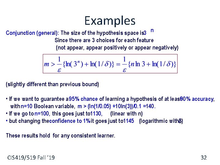
Examples Conjunction (general): The size of the hypothesis space is 3 n Since there are 3 choices for each feature (not appear, appear positively or appear negatively) (slightly different than previous bound) • If we want to guarantee a 95% chance of learning a hypothesis of at least 90% accuracy, with n=10 Boolean variable, m > (ln(1/0. 05) +10 ln(3))/0. 1 =140. • If we go to n=100, this goes just to 1130, (linear with n) • but changing theconfidence to 1% it goes just to 1145 (logarithmic with ) These results hold for any consistent learner. CIS 419/519 Fall ’ 19 32

Why Should We Care? § We now have a theory of generalization § § We know what are the important complexity parameters We understand the dependence in the number of examples and in the size of the hypothesis class § We have a generic procedure for learning that is guaranteed to generalize well § § § Draw a sample of size m. Develop an algorithm that is consistent with it. It will be good. § We have tools to prove that some hypothesis classes are learnable and some are not CIS 419/519 Fall ’ 19 33

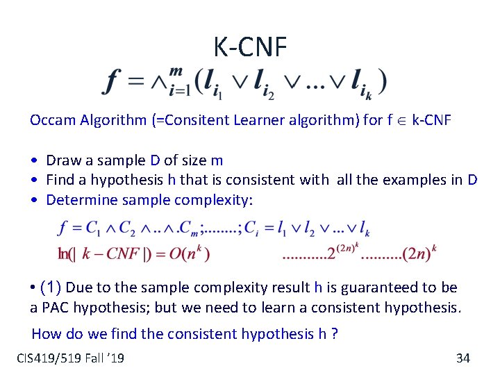
K-CNF Occam Algorithm (=Consitent Learner algorithm) for f k-CNF • Draw a sample D of size m • Find a hypothesis h that is consistent with all the examples in D • Determine sample complexity: • (1) Due to the sample complexity result h is guaranteed to be a PAC hypothesis; but we need to learn a consistent hypothesis. How do we find the consistent hypothesis h ? CIS 419/519 Fall ’ 19 34

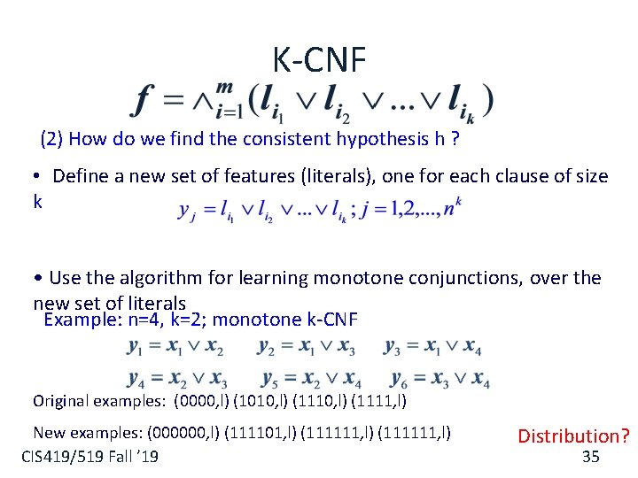
K-CNF (2) How do we find the consistent hypothesis h ? • Define a new set of features (literals), one for each clause of size k • Use the algorithm for learning monotone conjunctions, over the new set of literals Example: n=4, k=2; monotone k-CNF Original examples: (0000, l) (1010, l) (1111, l) New examples: (000000, l) (111101, l) (111111, l) CIS 419/519 Fall ’ 19 Distribution? 35

Negative Results – Examples § Two types of non-learnability results: § Complexity Theoretic § § Showing that various concepts classes cannot be learned, based on well-accepted assumptions from computational complexity theory. E. g. : C cannot be learned unless P=NP § Information Theoretic § § § The concept class is sufficiently rich that a polynomial number of examples may not be sufficient to distinguish a particular target concept. Both type involve “representation dependent” arguments. The proof shows that a given class cannot be learned by algorithms using hypotheses from the same class. (So? ) § Usually proofs are for EXACT learning, but apply for the distribution free case. CIS 419/519 Fall ’ 19 40

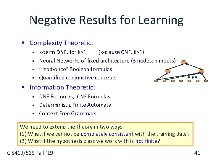
Negative Results for Learning § Complexity Theoretic: § § k-term DNF, for k>1 (k-clause CNF, k>1) Neural Networks of fixed architecture (3 nodes; n inputs) “read-once” Boolean formulas Quantified conjunctive concepts § Information Theoretic: § § § DNF Formulas; CNF Formulas Deterministic Finite Automata Context Free Grammars We need to extend theory in two ways: (1) What if we cannot be completely consistent with the training data? (2) What if the hypothesis class we work with is not finite? CIS 419/519 Fall ’ 19 41

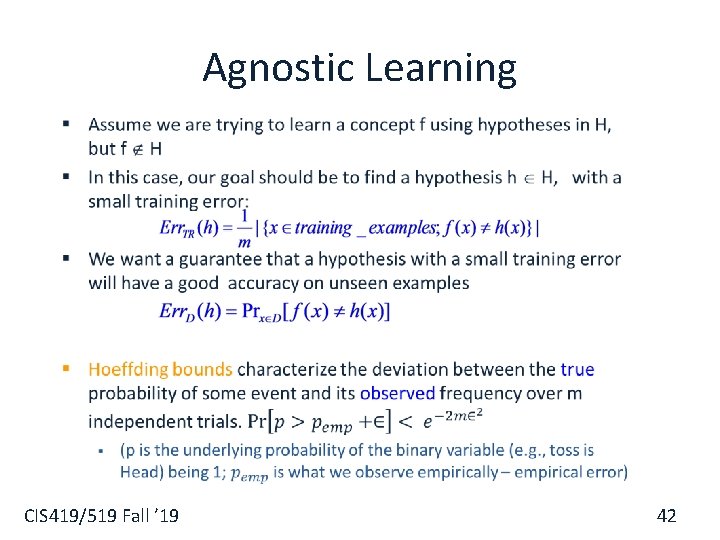
Agnostic Learning § CIS 419/519 Fall ’ 19 42

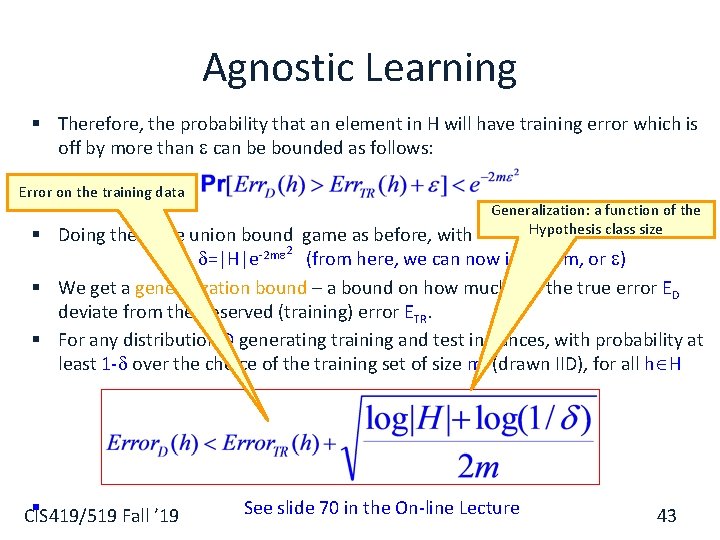
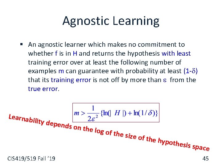
Agnostic Learning § Therefore, the probability that an element in H will have training error which is off by more than can be bounded as follows: Error on the training data Generalization: a function of the Hypothesis class size § Doing the same union bound game as before, with 2 =|H|e-2 m (from here, we can now isolate m, or ) § We get a generalization bound – a bound on how much will the true error ED deviate from the observed (training) error ETR. § For any distribution D generating training and test instances, with probability at least 1 - over the choice of the training set of size m, (drawn IID), for all h H § See slide 70 in the On-line Lecture CIS 419/519 Fall ’ 19 43

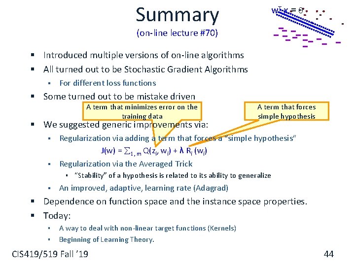
Summary w. T x = - ------ - - - (on-line lecture #70) § Introduced multiple versions of on-line algorithms § All turned out to be Stochastic Gradient Algorithms § For different loss functions § Some turned out to be mistake driven A term that minimizes error on the training data § We suggested generic improvements via: § § Regularization via adding a term that forces a “simple hypothesis” J(w) = 1, m Q(zi, wi) + λ Ri (wi) Regularization via the Averaged Trick § § A term that forces simple hypothesis “Stability” of a hypothesis is related to its ability to generalize An improved, adaptive, learning rate (Adagrad) § Dependence on function space and the instance space properties. § Today: § § A way to deal with non-linear target functions (Kernels) Beginning of Learning Theory. CIS 419/519 Fall ’ 19 44

Agnostic Learning § An agnostic learner which makes no commitment to whether f is in H and returns the hypothesis with least training error over at least the following number of examples m can guarantee with probability at least (1 - ) that its training error is not off by more than from the true error. Learnab ility dep CIS 419/519 Fall ’ 19 ends on the log o f the siz e of the hypothe sis space 45

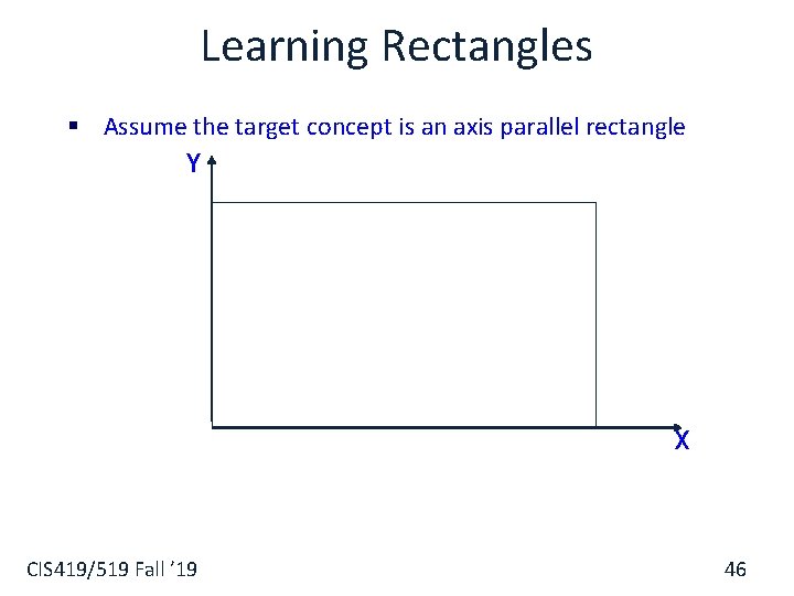
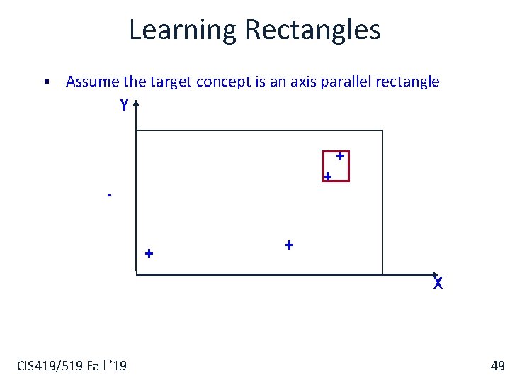
Learning Rectangles § Assume the target concept is an axis parallel rectangle Y X CIS 419/519 Fall ’ 19 46

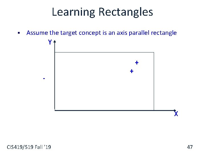
Learning Rectangles § Assume the target concept is an axis parallel rectangle Y + - + X CIS 419/519 Fall ’ 19 47

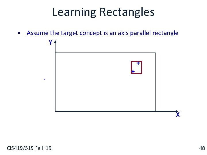
Learning Rectangles § Assume the target concept is an axis parallel rectangle Y + - + X CIS 419/519 Fall ’ 19 48

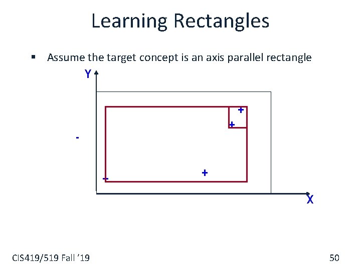
Learning Rectangles § Assume the target concept is an axis parallel rectangle Y + + X CIS 419/519 Fall ’ 19 49

Learning Rectangles § Assume the target concept is an axis parallel rectangle Y + + X CIS 419/519 Fall ’ 19 50

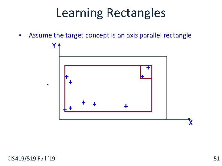
Learning Rectangles § Assume the target concept is an axis parallel rectangle Y + - + ++ + X CIS 419/519 Fall ’ 19 51

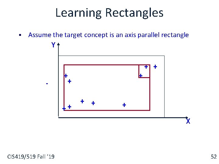
Learning Rectangles § Assume the target concept is an axis parallel rectangle Y + + - + ++ + X CIS 419/519 Fall ’ 19 52

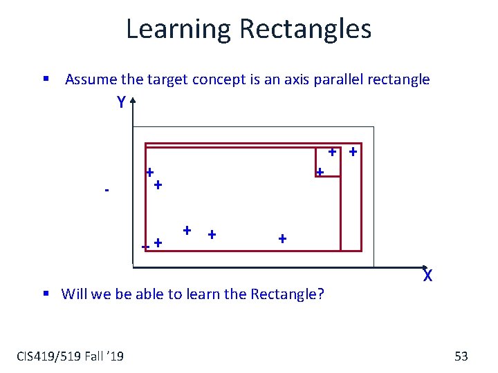
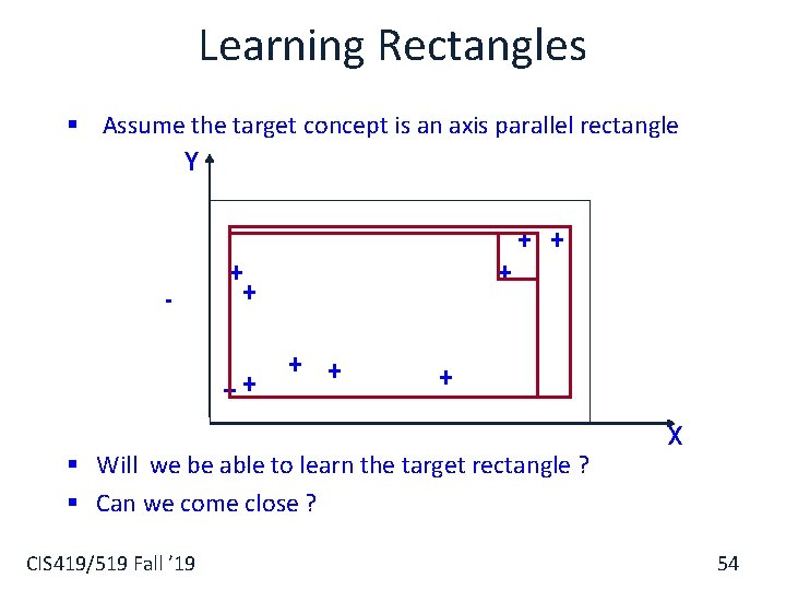
Learning Rectangles § Assume the target concept is an axis parallel rectangle Y + + - + ++ + § Will we be able to learn the Rectangle? CIS 419/519 Fall ’ 19 X 53

Learning Rectangles § Assume the target concept is an axis parallel rectangle Y + + - + ++ + § Will we be able to learn the target rectangle ? § Can we come close ? CIS 419/519 Fall ’ 19 X 54

Infinite Hypothesis Space § The previous analysis was restricted to finite hypothesis spaces § Some infinite hypothesis spaces are more expressive than others § § E. g. , Rectangles, vs. 17 - sides convex polygons vs. general convex polygons Linear threshold function vs. a conjunction of LTUs § Need a measure of the expressiveness of an infinite hypothesis space other than its size § The Vapnik-Chervonenkis dimension (VC dimension) provides such a measure. § Analogous to |H|, there are bounds for sample complexity using VC(H) CIS 419/519 Fall ’ 19 55

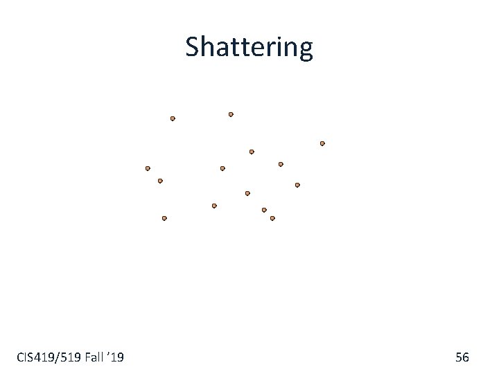
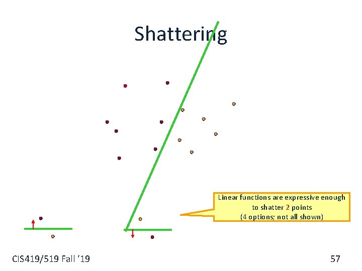
Shattering CIS 419/519 Fall ’ 19 56

Shattering Linear functions are expressive enough to shatter 2 points (4 options; not all shown) CIS 419/519 Fall ’ 19 57

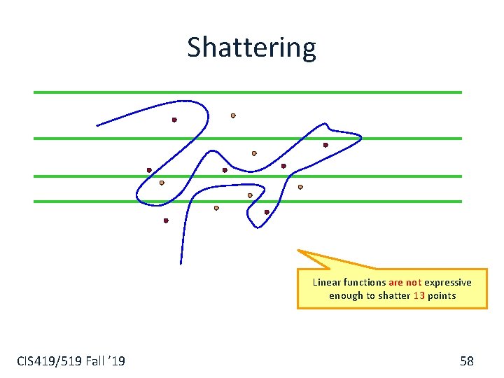
Shattering Linear functions are not expressive enough to shatter 13 points CIS 419/519 Fall ’ 19 58

Shattering • We say that a set S of examples is shattered by a set of functions H if for every partition of the examples in S into positive and negative examples there is a function in H that gives exactly these labels to the examples (Intuition: A rich set of functions shatters large sets of points) CIS 419/519 Fall ’ 19 59

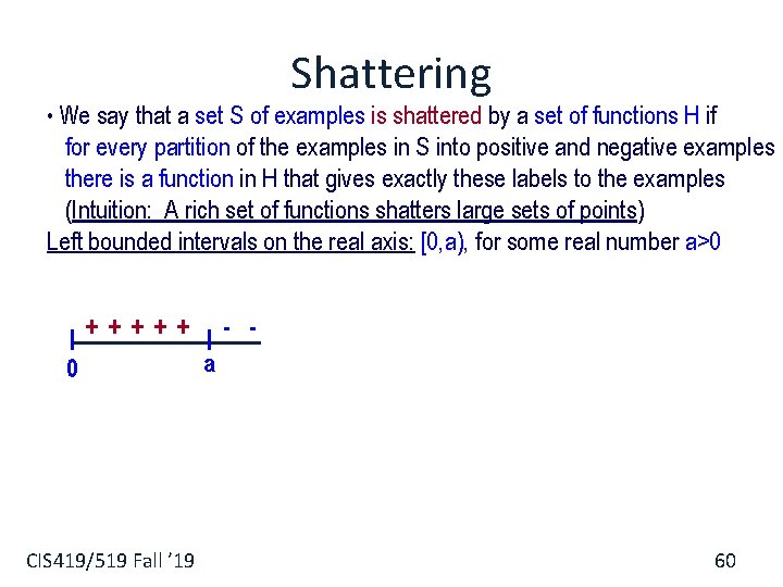
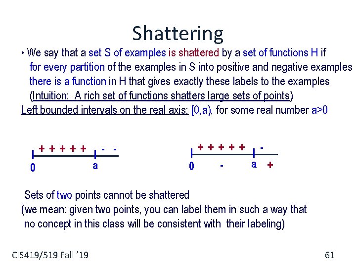
Shattering • We say that a set S of examples is shattered by a set of functions H if for every partition of the examples in S into positive and negative examples there is a function in H that gives exactly these labels to the examples (Intuition: A rich set of functions shatters large sets of points) Left bounded intervals on the real axis: [0, a), for some real number a>0 +++++ 0 CIS 419/519 Fall ’ 19 - a 60

Shattering • We say that a set S of examples is shattered by a set of functions H if for every partition of the examples in S into positive and negative examples there is a function in H that gives exactly these labels to the examples (Intuition: A rich set of functions shatters large sets of points) Left bounded intervals on the real axis: [0, a), for some real number a>0 +++++ 0 - a +++++ a + 0 Sets of two points cannot be shattered (we mean: given two points, you can label them in such a way that no concept in this class will be consistent with their labeling) CIS 419/519 Fall ’ 19 61

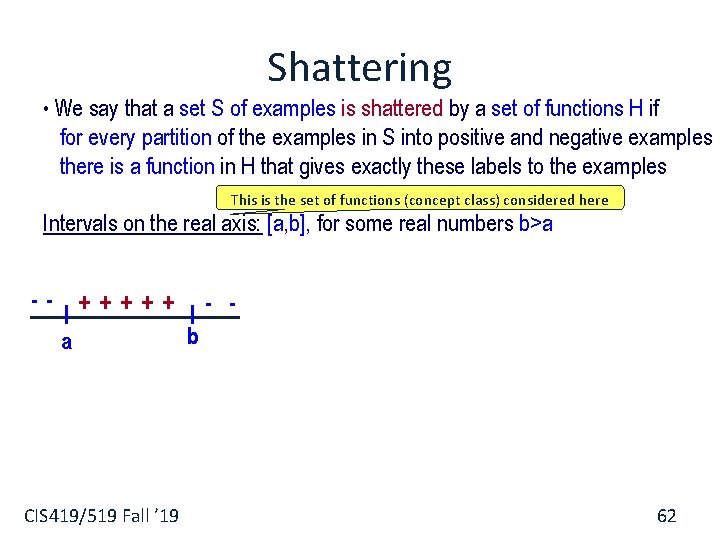
Shattering • We say that a set S of examples is shattered by a set of functions H if for every partition of the examples in S into positive and negative examples there is a function in H that gives exactly these labels to the examples This is the set of functions (concept class) considered here Intervals on the real axis: [a, b], for some real numbers b>a -- +++++ a CIS 419/519 Fall ’ 19 - b 62

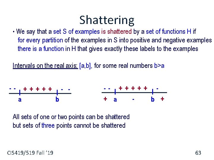
Shattering • We say that a set S of examples is shattered by a set of functions H if for every partition of the examples in S into positive and negative examples there is a function in H that gives exactly these labels to the examples Intervals on the real axis: [a, b], for some real numbers b>a -- +++++ a - b -- +++++ + a b + All sets of one or two points can be shattered but sets of three points cannot be shattered CIS 419/519 Fall ’ 19 63

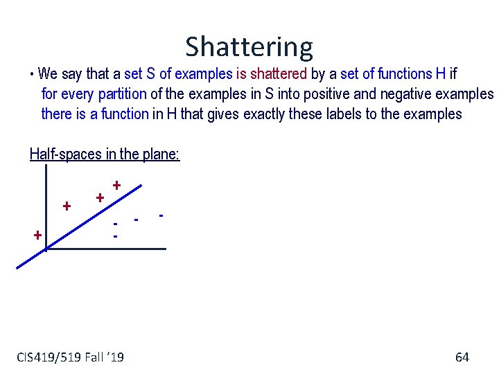
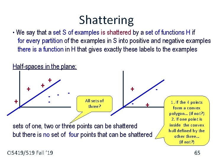
Shattering • We say that a set S of examples is shattered by a set of functions H if for every partition of the examples in S into positive and negative examples there is a function in H that gives exactly these labels to the examples Half-spaces in the plane: + + - - CIS 419/519 Fall ’ 19 - 64

Shattering • We say that a set S of examples is shattered by a set of functions H if for every partition of the examples in S into positive and negative examples there is a function in H that gives exactly these labels to the examples Half-spaces in the plane: + + - - + All sets of three? - + sets of one, two or three points can be shattered but there is no set of four points that can be shattered CIS 419/519 Fall ’ 19 1. If the 4 points form a convex polygon… (if not? ) 2. If one point is inside the convex hull defined by the other three… (if not? ) 65

VC Dimension • An unbiased hypothesis space H shatters the entire instance space X, i. e, it is able to induce every possible partition on the set of all possible instances. • The larger the subset X that can be shattered, the more expressive a hypothesis space is, i. e. , the less biased. CIS 419/519 Fall ’ 19 66

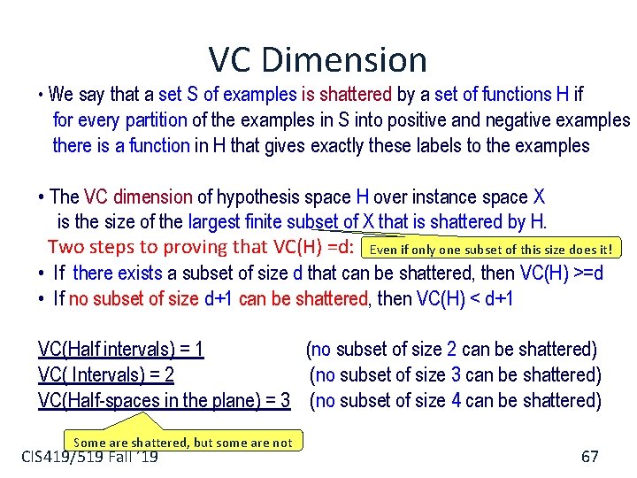
VC Dimension • We say that a set S of examples is shattered by a set of functions H if for every partition of the examples in S into positive and negative examples there is a function in H that gives exactly these labels to the examples • The VC dimension of hypothesis space H over instance space X is the size of the largest finite subset of X that is shattered by H. Two steps to proving that VC(H) =d: Even if only one subset of this size does it! • If there exists a subset of size d that can be shattered, then VC(H) >=d • If no subset of size d+1 can be shattered, then VC(H) < d+1 VC(Half intervals) = 1 (no subset of size 2 can be shattered) VC( Intervals) = 2 (no subset of size 3 can be shattered) VC(Half-spaces in the plane) = 3 (no subset of size 4 can be shattered) Some are shattered, but some are not CIS 419/519 Fall ’ 19 67

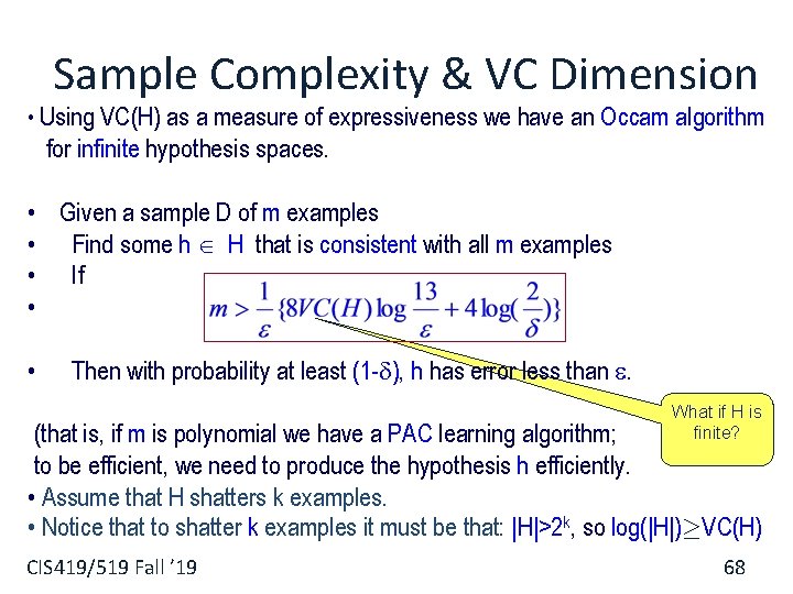
Sample Complexity & VC Dimension • Using VC(H) as a measure of expressiveness we have an Occam algorithm for infinite hypothesis spaces. • Given a sample D of m examples • Find some h H that is consistent with all m examples • If • • Then with probability at least (1 - ), h has error less than . What if H is finite? (that is, if m is polynomial we have a PAC learning algorithm; to be efficient, we need to produce the hypothesis h efficiently. • Assume that H shatters k examples. • Notice that to shatter k examples it must be that: |H|>2 k, so log(|H|)¸VC(H) CIS 419/519 Fall ’ 19 68

Learning Rectangles • Consider axis parallel rectangles in the real plan • Can we PAC learn it ? CIS 419/519 Fall ’ 19 69

Learning Rectangles • Consider axis parallel rectangles in the real plan • Can we PAC learn it ? (1) What is the VC dimension ? CIS 419/519 Fall ’ 19 70

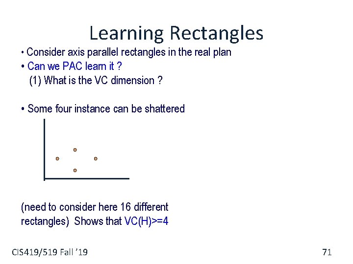
Learning Rectangles • Consider axis parallel rectangles in the real plan • Can we PAC learn it ? (1) What is the VC dimension ? • Some four instance can be shattered (need to consider here 16 different rectangles) Shows that VC(H)>=4 CIS 419/519 Fall ’ 19 71

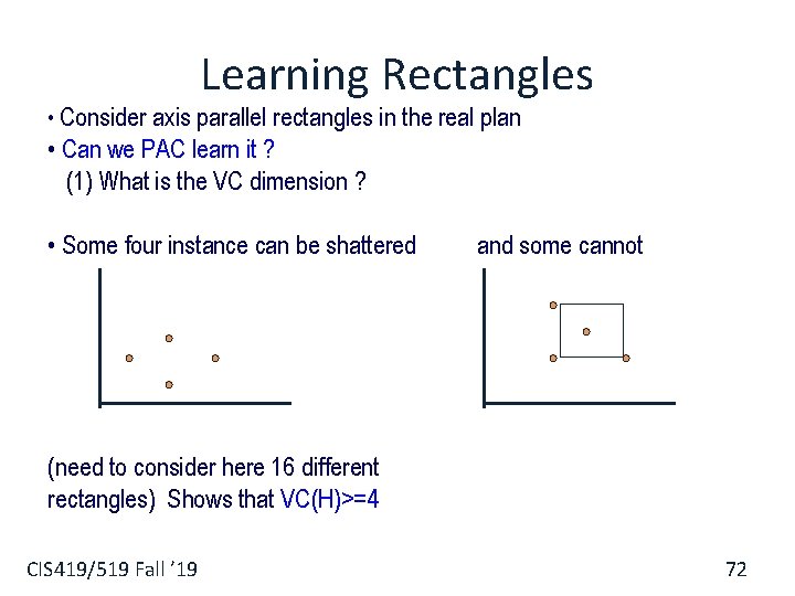
Learning Rectangles • Consider axis parallel rectangles in the real plan • Can we PAC learn it ? (1) What is the VC dimension ? • Some four instance can be shattered and some cannot (need to consider here 16 different rectangles) Shows that VC(H)>=4 CIS 419/519 Fall ’ 19 72

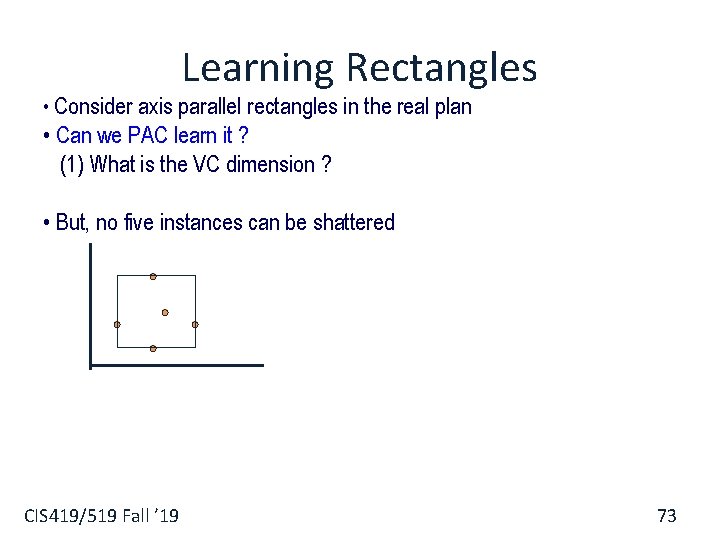
Learning Rectangles • Consider axis parallel rectangles in the real plan • Can we PAC learn it ? (1) What is the VC dimension ? • But, no five instances can be shattered CIS 419/519 Fall ’ 19 73

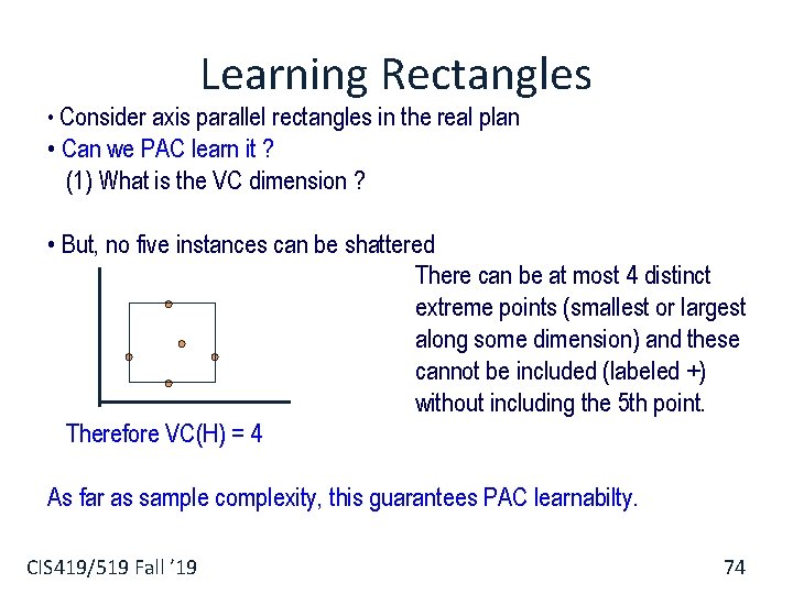
Learning Rectangles • Consider axis parallel rectangles in the real plan • Can we PAC learn it ? (1) What is the VC dimension ? • But, no five instances can be shattered There can be at most 4 distinct extreme points (smallest or largest along some dimension) and these cannot be included (labeled +) without including the 5 th point. Therefore VC(H) = 4 As far as sample complexity, this guarantees PAC learnabilty. CIS 419/519 Fall ’ 19 74

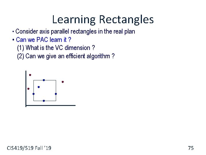
Learning Rectangles • Consider axis parallel rectangles in the real plan • Can we PAC learn it ? (1) What is the VC dimension ? (2) Can we give an efficient algorithm ? CIS 419/519 Fall ’ 19 75

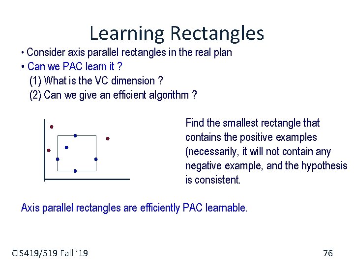
Learning Rectangles • Consider axis parallel rectangles in the real plan • Can we PAC learn it ? (1) What is the VC dimension ? (2) Can we give an efficient algorithm ? Find the smallest rectangle that contains the positive examples (necessarily, it will not contain any negative example, and the hypothesis is consistent. Axis parallel rectangles are efficiently PAC learnable. CIS 419/519 Fall ’ 19 76

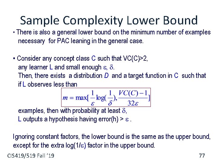
Sample Complexity Lower Bound • There is also a general lower bound on the minimum number of examples necessary for PAC leaning in the general case. • Consider any concept class C such that VC(C)>2, any learner L and small enough , . Then, there exists a distribution D and a target function in C such that if L observes less than examples, then with probability at least , L outputs a hypothesis having error(h) > . Ignoring constant factors, the lower bound is the same as the upper bound, except for the extra log(1/ ) factor in the upper bound. CIS 419/519 Fall ’ 19 77

COLT Conclusions § The PAC framework provides a reasonable model for theoretically analyzing the effectiveness of learning algorithms. § The sample complexity for any consistent learner using the hypothesis space, H, can be determined from a measure of H’s expressiveness (|H|, VC(H)) § If the sample complexity is tractable, then the computational complexity of finding a consistent hypothesis governs the complexity of the problem. § Sample complexity bounds given here are far from being tight, but separate learnable classes from non-learnable classes (and show what’s important). They also guide us to try and use smaller hypothesis spaces. § Computational complexity results exhibit cases where information theoretic learning is feasible, but finding good hypothesis is intractable. § The theoretical framework allows for a concrete analysis of the complexity of learning as a function of various assumptions (e. g. , relevant variables) CIS 419/519 Fall ’ 19 78

COLT Conclusions (2) § Many additional models have been studied as extensions of the basic one: § § § § Learning with noisy data Learning under specific distributions Learning probabilistic representations Learning neural networks Learning finite automata Active Learning; Learning with Queries Models of Teaching § An important extension: PAC-Bayesians theory. § In addition to the Distribution Free assumption of PAC, makes also an assumption of a prior distribution over the hypothesis the learner can choose from. CIS 419/519 Fall ’ 19 79

COLT Conclusions (3) § Theoretical results shed light on important issues such as the importance of the bias (representation), sample and computational complexity, importance of interaction, etc. § Bounds guide model selection even when not practical. § A lot of recent work is on data dependent bounds. § The impact COLT has had on practical learning system in the last few years has been very significant: § § SVMs; Winnow (Sparsity), Boosting Regularization CIS 419/519 Fall ’ 19 80