CIS 519419 Applied Machine Learning www seas upenn

CIS 519/419 Applied Machine Learning www. seas. upenn. edu/~cis 519 Dan Roth danroth@seas. upenn. edu http: //www. cis. upenn. edu/~danroth/ 461 C, 3401 Walnut Slides were created by Dan Roth (for CIS 519/419 at Penn or CS 446 at UIUC), Eric Eaton for CIS 519/419 at Penn, or from other authors who have made their ML slides available. CIS 419/519 Spring ’ 18

Administration § Exam: § The exam will take place on the originally assigned date, 4/30. § § § Similar to the previous midterm. 75 minutes; closed books. What is covered: § § The focus is on the material covered after the previous mid-term. However, notice that the ideas in this class are cumulative!! Everything that we present in class and in the homework assignments Material that is in the slides but is not discussed in class is not part of the material required for the exam. • Example 1: We talked about Boosting. But not about boosting the confidence. • Example 2: We talked about multiclassification: Ov. A, Av. A, but not Error Correcting codes, and additional material in the slides. § We will give a few practice exams. CIS 419/519 Spring ’ 18 2

Administration § Projects § We will have a poster session 6 -8 pm on May 7 § § § § in the active learning room, 3401 Walnut. (72% of the CIS 519 students that voted in our poll preferred that). The hope is that this will be a fun event where all of you have an opportunity to see and discuss the projects people have done. All are invited! Mandatory for CIS 519 students The final project report will be due on 5/8 Logistics: you will send us you posters the a day earlier; we will print it and hang it; you will present it. § If you haven’t done so already: § Come to my office hours at least once this or next week to discuss the project!! Go to Bayes CIS 419/519 Spring ’ 18 3

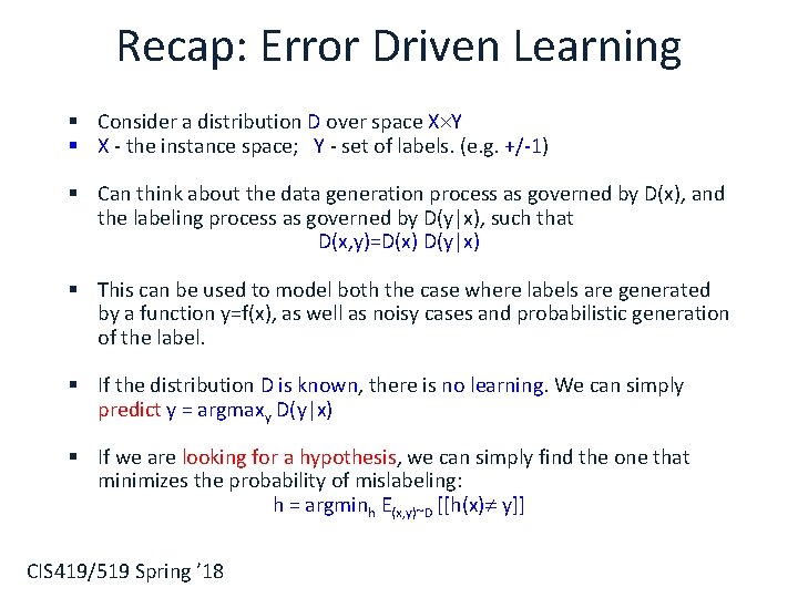
Recap: Error Driven Learning § Consider a distribution D over space X Y § X - the instance space; Y - set of labels. (e. g. +/-1) § Can think about the data generation process as governed by D(x), and the labeling process as governed by D(y|x), such that D(x, y)=D(x) D(y|x) § This can be used to model both the case where labels are generated by a function y=f(x), as well as noisy cases and probabilistic generation of the label. § If the distribution D is known, there is no learning. We can simply predict y = argmaxy D(y|x) § If we are looking for a hypothesis, we can simply find the one that minimizes the probability of mislabeling: h = argminh E(x, y)~D [[h(x) y]] CIS 419/519 Spring ’ 18

Recap: Error Driven Learning (2) § Inductive learning comes into play when the distribution is not known. § Then, there are two basic approaches to take. § Discriminative (direct) learning § and § Bayesian Learning (Generative) § Running example: Text Correction: § “I saw the girl it the park” I saw the girl in the park CIS 419/519 Spring ’ 18 5

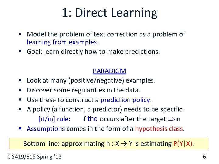
1: Direct Learning § Model the problem of text correction as a problem of learning from examples. § Goal: learn directly how to make predictions. § § § PARADIGM Look at many (positive/negative) examples. Discover some regularities in the data. Use these to construct a prediction policy. A policy (a function, a predictor) needs to be specific. [it/in] rule: if the occurs after the target in Assumptions comes in the form of a hypothesis class. Bottom line: approximating h : X → Y is estimating P(Y|X). CIS 419/519 Spring ’ 18 6

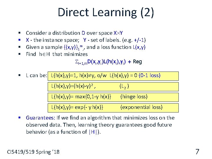
Direct Learning (2) § § Consider a distribution D over space X Y X - the instance space; Y - set of labels. (e. g. +/-1) Given a sample {(x, y)}1 m, , and a loss function L(x, y) Find h H that minimizes i=1, m. D(xi, yi)L(h(xi), yi) + Reg § L can be: L(h(x), y)=1, h(x) y, o/w L(h(x), y) = 0 (0 -1 loss) L(h(x), y)=(h(x)-y)2 , (L 2 ) L(h(x), y)= max{0, 1 -y h(x)} (hinge loss) L(h(x), y)= exp{- y h(x)} (exponential loss) § Guarantees: If we find an algorithm that minimizes loss on the observed data. Then, learning theory guarantees good future behavior (as a function of |H|). CIS 419/519 Spring ’ 18 7

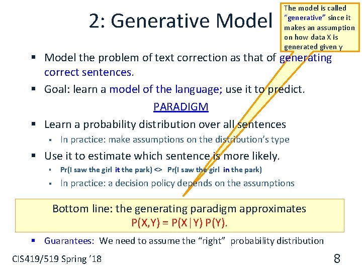
2: Generative Model The model is called “generative” since it makes an assumption on how data X is generated given y § Model the problem of text correction as that of generating correct sentences. § Goal: learn a model of the language; use it to predict. PARADIGM § Learn a probability distribution over all sentences § In practice: make assumptions on the distribution’s type § Use it to estimate which sentence is more likely. § Pr(I saw the girl it the park) <> Pr(I saw the girl in the park) § In practice: a decision policy depends on the assumptions Bottom line: the generating paradigm approximates P(X, Y) = P(X|Y) P(Y). § Guarantees: We need to assume the “right” probability distribution CIS 419/519 Spring ’ 18 8

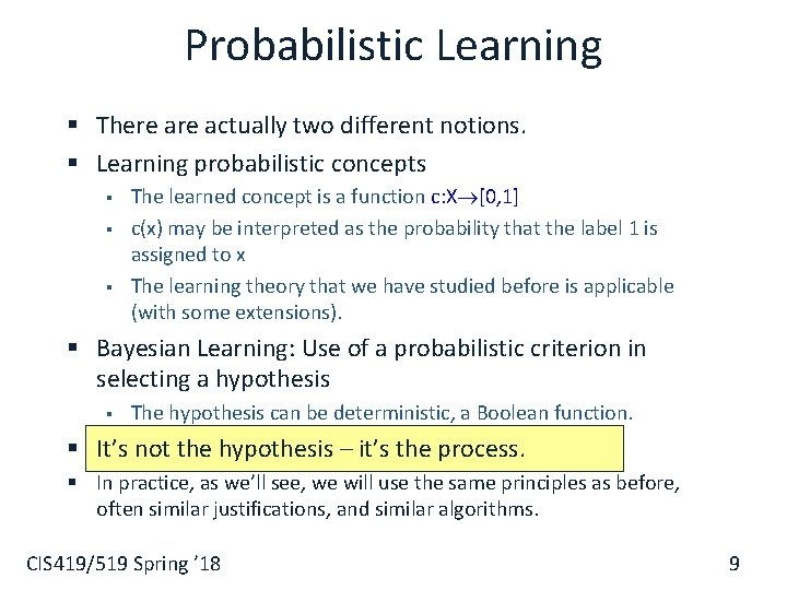
Probabilistic Learning § There actually two different notions. § Learning probabilistic concepts § § § The learned concept is a function c: X [0, 1] c(x) may be interpreted as the probability that the label 1 is assigned to x The learning theory that we have studied before is applicable (with some extensions). § Bayesian Learning: Use of a probabilistic criterion in selecting a hypothesis § The hypothesis can be deterministic, a Boolean function. § It’s not the hypothesis – it’s the process. § In practice, as we’ll see, we will use the same principles as before, often similar justifications, and similar algorithms. CIS 419/519 Spring ’ 18 9

Probabilities § 30 years of AI research danced around the fact that the world was inherently uncertain § Bayesian Inference: § § § Use probability theory and information about independence Reason diagnostically (from evidence (effects) to conclusions (causes)). . . or causally (from causes to effects) § Probabilistic reasoning only gives probabilistic results § i. e. , it summarizes uncertainty from various sources § We will only use it as a tool in Machine Learning. CIS 419/519 Spring ’ 18

Concepts § § Probability, Probability Space and Events Joint Events Conditional Probabilities Independence § § Go to the recitation on Tuesday/Thursday Use the material we provided on-line § Next I will give a very quick refresher CIS 419/519 Spring ’ 18 11

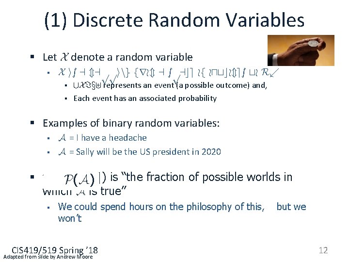
(1) Discrete Random Variables § Let X denote a random variable § X is a mapping from a space of outcomes to R. § § [X=x] represents an event (a possible outcome) and, Each event has an associated probability § Examples of binary random variables: § § A = I have a headache A = Sally will be the US president in 2020 § P(A=True) P(A) is “the fraction of possible worlds in which A is true” § We could spend hours on the philosophy of this, won’t CIS 419/519 Spring ’ 18 Adapted from slide by Andrew Moore but we 12

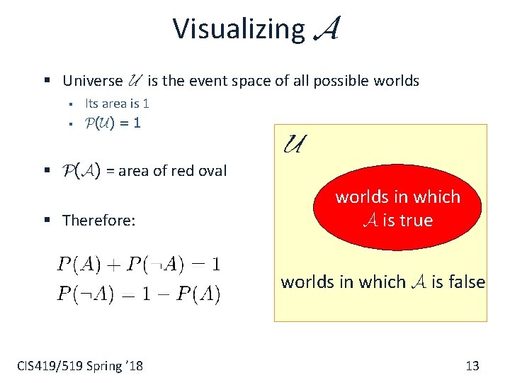
Visualizing A § Universe U is the event space of all possible worlds § § Its area is 1 P(U) = 1 U § P(A) = area of red oval § Therefore: worlds in which A is true worlds in which A is false CIS 419/519 Spring ’ 18 13

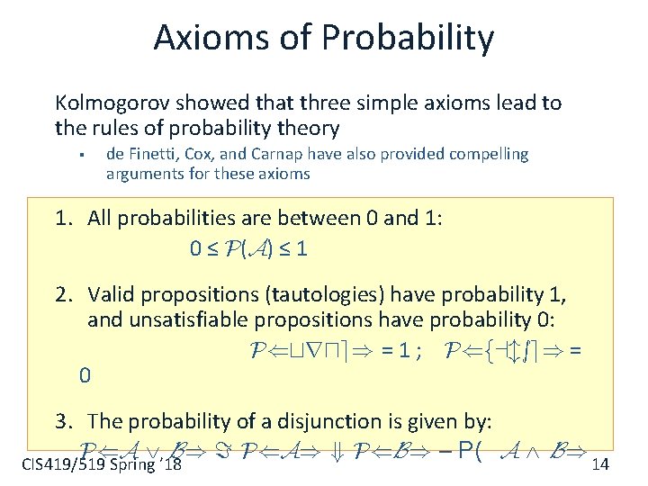
Axioms of Probability Kolmogorov showed that three simple axioms lead to the rules of probability theory § de Finetti, Cox, and Carnap have also provided compelling arguments for these axioms 1. All probabilities are between 0 and 1: 0 ≤ P(A) ≤ 1 2. Valid propositions (tautologies) have probability 1, and unsatisfiable propositions have probability 0: P(true) = 1 ; P(false) = 0 3. The probability of a disjunction is given by: P(A B) = P(A) + P(B) – P( A B) 14 CIS 419/519 Spring ’ 18

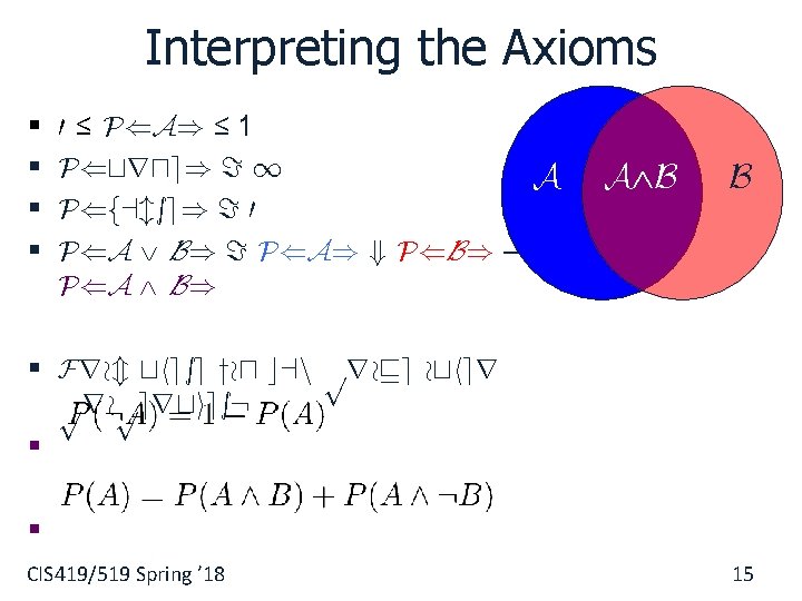
Interpreting the Axioms § § 0 ≤ P(A) ≤ 1 P(true) = 1 P(false) = 0 P(A B) = P(A) + P(B) – P(A B) A A B B § From these you can prove other properties: § § CIS 419/519 Spring ’ 18 15

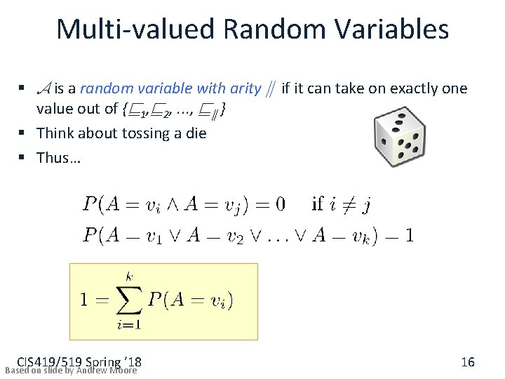
Multi-valued Random Variables § A is a random variable with arity k if it can take on exactly one value out of {v 1, v 2, . . . , vk } § Think about tossing a die § Thus… CIS 419/519 Spring ’ 18 Based on slide by Andrew Moore 16

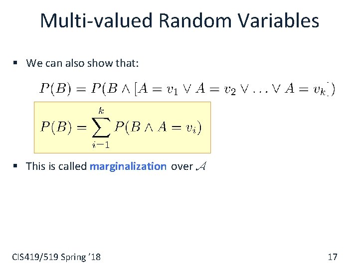
Multi-valued Random Variables § We can also show that: § This is called marginalization over A CIS 419/519 Spring ’ 18 17

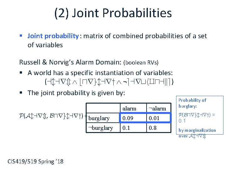
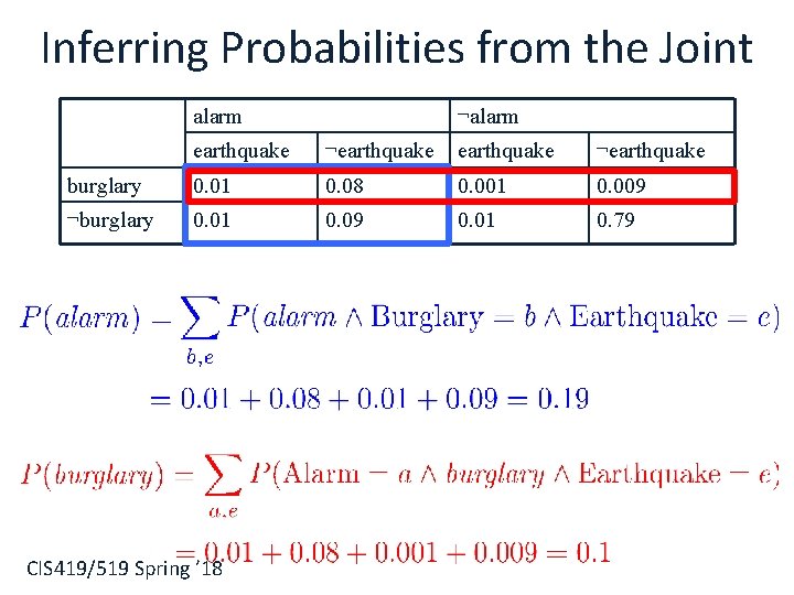
(2) Joint Probabilities § Joint probability: matrix of combined probabilities of a set of variables Russell & Norvig’s Alarm Domain: (boolean RVs) § A world has a specific instantiation of variables: (alarm burglary ¬earthquake) § The joint probability is given by: P(Alarm, Burglary) = burglary ¬burglary CIS 419/519 Spring ’ 18 alarm ¬alarm 0. 09 0. 01 0. 8 Probability of burglary: P(Burglary) = 0. 1 by marginalization over Alarm

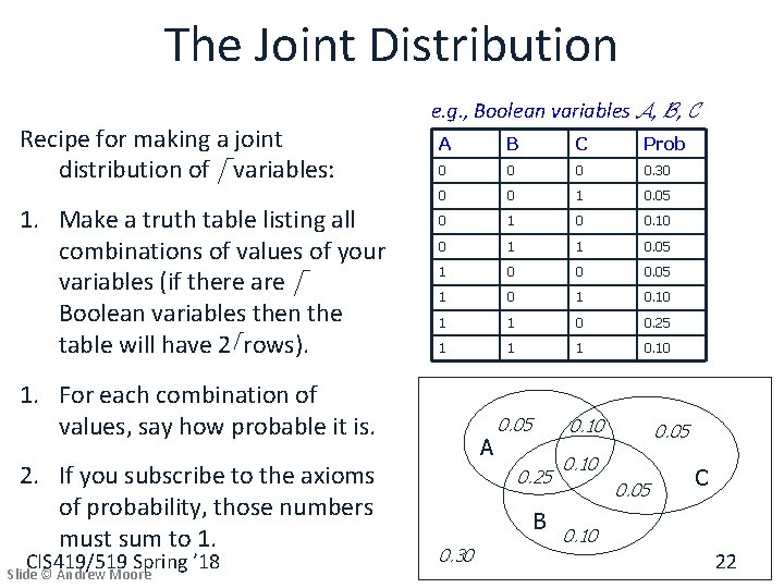
The Joint Distribution Recipe for making a joint distribution of d variables: CIS 419/519 Spring ’ 18 Slide © Andrew Moore e. g. , Boolean variables A, B, C 19

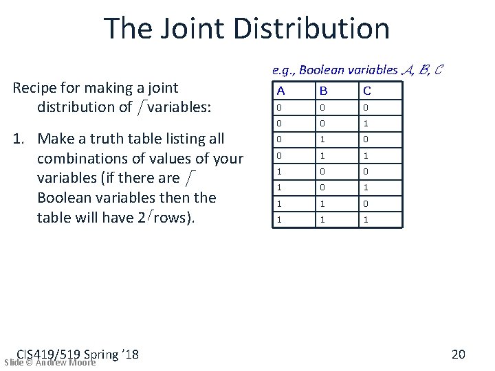
The Joint Distribution Recipe for making a joint distribution of d variables: 1. Make a truth table listing all combinations of values of your variables (if there are d Boolean variables then the table will have 2 d rows). CIS 419/519 Spring ’ 18 Slide © Andrew Moore e. g. , Boolean variables A, B, C A B C 0 0 0 1 1 1 0 0 1 1 1 20

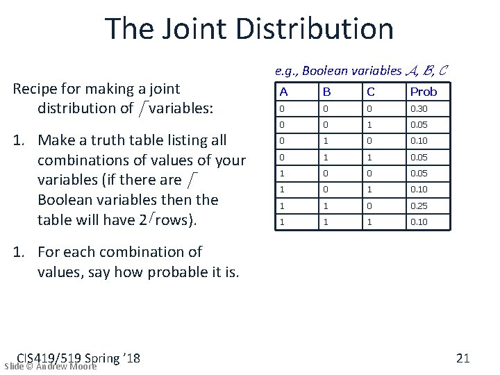
The Joint Distribution Recipe for making a joint distribution of d variables: 1. Make a truth table listing all combinations of values of your variables (if there are d Boolean variables then the table will have 2 d rows). e. g. , Boolean variables A, B, C A B C Prob 0 0. 30 0 0 1 0. 05 0 1 0 0. 10 0 1 1 0. 05 1 0 0 0. 05 1 0. 10 1 1 0 0. 25 1 1 1 0. 10 1. For each combination of values, say how probable it is. CIS 419/519 Spring ’ 18 Slide © Andrew Moore 21

The Joint Distribution Recipe for making a joint distribution of d variables: 1. Make a truth table listing all combinations of values of your variables (if there are d Boolean variables then the table will have 2 d rows). e. g. , Boolean variables A, B, C A B C Prob 0 0. 30 0 0 1 0. 05 0 1 0 0. 10 0 1 1 0. 05 1 0 0 0. 05 1 0. 10 1 1 0 0. 25 1 1 1 0. 10 1. For each combination of values, say how probable it is. 2. If you subscribe to the axioms of probability, those numbers must sum to 1. CIS 419/519 Spring ’ 18 Slide © Andrew Moore A 0. 05 0. 10 0. 25 B 0. 30 0. 05 0. 10 0. 05 C 0. 10 22

Inferring Probabilities from the Joint alarm ¬alarm earthquake ¬earthquake burglary 0. 01 0. 08 0. 001 0. 009 ¬burglary 0. 01 0. 09 0. 01 0. 79 CIS 419/519 Spring ’ 18

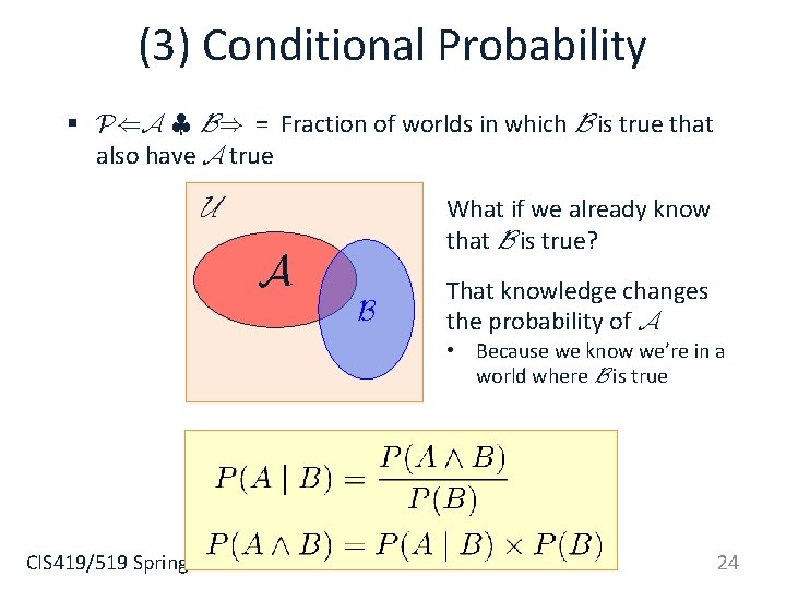
(3) Conditional Probability § P(A | B) = Fraction of worlds in which B is true that also have A true U A What if we already know that B is true? B That knowledge changes the probability of A • Because we know we’re in a world where B is true CIS 419/519 Spring ’ 18 24

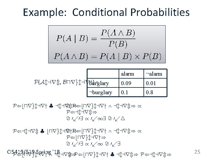
Example: Conditional Probabilities P(Alarm, Burglary) = burglary ¬burglary alarm ¬alarm 0. 09 0. 01 0. 8 = P(burglary alarm) / P(burglary | alarm) P(alarm) = 0. 09 / 0. 19 = 0. 4 = P(burglary alarm) / P(alarm | burglary) P(burglary) = 0. 09 / 0. 1 = 0. 9 CIS 419/519 Spring ’ 18 = P(burglary | alarm) P(burglary alarm) 25

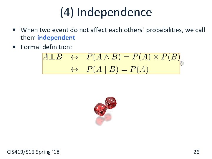
(4) Independence § When two event do not affect each others’ probabilities, we call them independent § Formal definition: CIS 419/519 Spring ’ 18 26

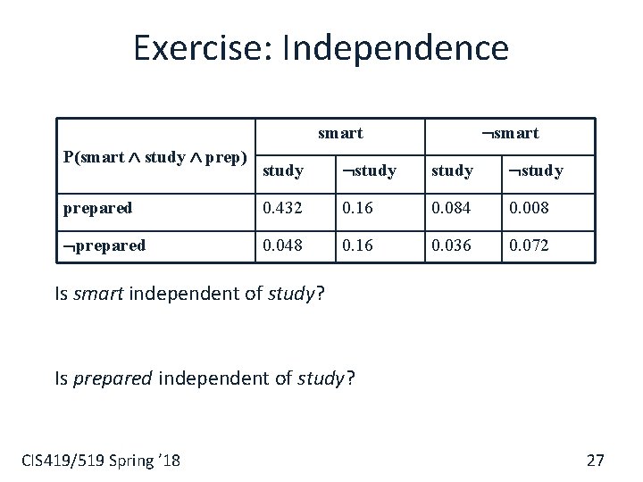
Exercise: Independence smart P(smart study prep) study prepared 0. 432 0. 16 0. 084 0. 008 prepared 0. 048 0. 16 0. 036 0. 072 Is smart independent of study? Is prepared independent of study? CIS 419/519 Spring ’ 18 27

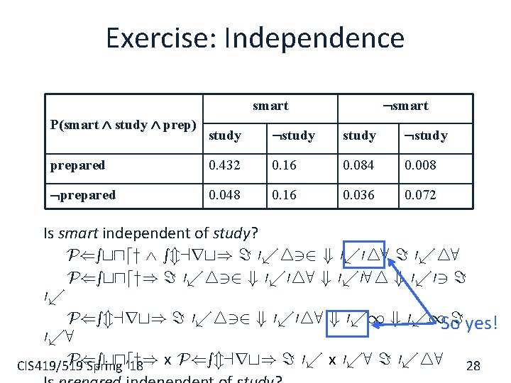
Exercise: Independence smart P(smart study prep) study prepared 0. 432 0. 16 0. 084 0. 008 prepared 0. 048 0. 16 0. 036 0. 072 Is smart independent of study? P(study smart) = 0. 432 + 0. 048 = 0. 48 P(study) = 0. 432 + 0. 048 + 0. 084 + 0. 03 = 0. P(smart) = 0. 432 + 0. 048 + 0. 1 So = yes! 0. 8 P(study) 28 CIS 419/519 Spring ’ 18 x P(smart) = 0. x 0. 8 = 0. 48

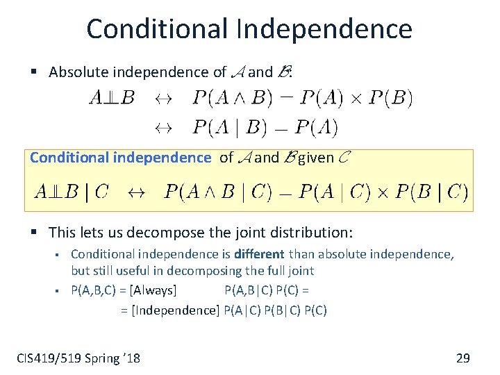
Conditional Independence § Absolute independence of A and B: Conditional independence of A and B given C § This lets us decompose the joint distribution: § § Conditional independence is different than absolute independence, but still useful in decomposing the full joint P(A, B, C) = [Always] P(A, B|C) P(C) = = [Independence] P(A|C) P(B|C) P(C) CIS 419/519 Spring ’ 18 29

Exercise: Independence smart P(smart study prep) study prepared 0. 432 0. 16 0. 084 0. 008 prepared 0. 048 0. 16 0. 036 0. 072 Is smart independent of study? Is prepared independent of study? CIS 419/519 Spring ’ 18 30

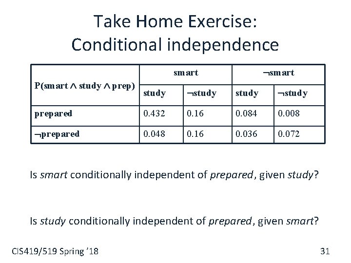
Take Home Exercise: Conditional independence smart P(smart study prep) study prepared 0. 432 0. 16 0. 084 0. 008 prepared 0. 048 0. 16 0. 036 0. 072 Is smart conditionally independent of prepared, given study? Is study conditionally independent of prepared, given smart? CIS 419/519 Spring ’ 18 31

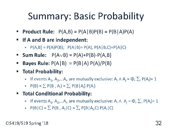
Summary: Basic Probability § CIS 419/519 Spring ’ 18 32

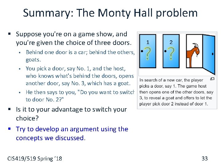
Summary: The Monty Hall problem § Suppose you're on a game show, and you're given the choice of three doors. § § § Behind one door is a car; behind the others, goats. You pick a door, say No. 1, and the host, who knows what's behind the doors, opens another door, say No. 3, which has a goat. He then says to you, "Do you want to switch to door No. 2? " § Is it to your advantage to switch your choice? § Try to develop an argument using the concepts we discussed. CIS 419/519 Spring ’ 18 33

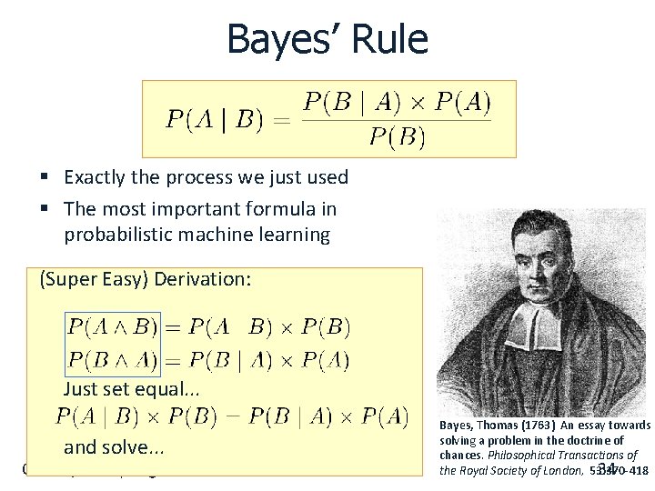
Bayes’ Rule § Exactly the process we just used § The most important formula in probabilistic machine learning (Super Easy) Derivation: Just set equal. . . and solve. . . CIS 419/519 Spring ’ 18 Bayes, Thomas (1763) An essay towards solving a problem in the doctrine of chances. Philosophical Transactions of 34 the Royal Society of London, 53: 370 -418

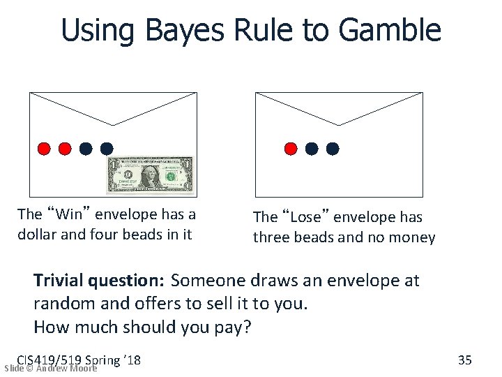
Using Bayes Rule to Gamble The “Win” envelope has a dollar and four beads in it The “Lose” envelope has three beads and no money Trivial question: Someone draws an envelope at random and offers to sell it to you. How much should you pay? CIS 419/519 Spring ’ 18 Slide © Andrew Moore 35

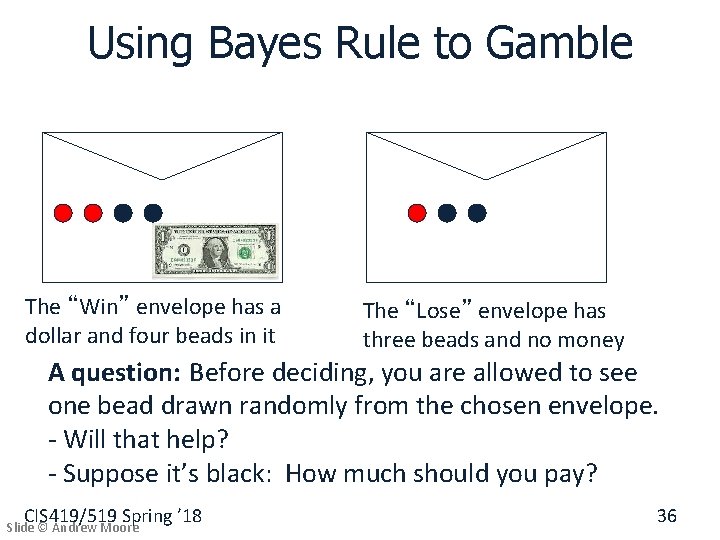
Using Bayes Rule to Gamble The “Win” envelope has a dollar and four beads in it The “Lose” envelope has three beads and no money A question: Before deciding, you are allowed to see one bead drawn randomly from the chosen envelope. - Will that help? - Suppose it’s black: How much should you pay? CIS 419/519 Spring ’ 18 Slide © Andrew Moore 36

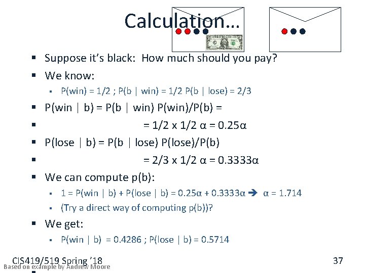
Calculation… § Suppose it’s black: How much should you pay? § We know: § P(win) = 1/2 ; P(b | win) = 1/2 P(b | lose) = 2/3 § P(win | b) = P(b | win) P(win)/P(b) = § = 1/2 x 1/2 α = 0. 25α § P(lose | b) = P(b | lose) P(lose)/P(b) § = 2/3 x 1/2 α = 0. 3333α § We can compute p(b): § § 1 = P(win | b) + P(lose | b) = 0. 25α + 0. 3333α α = 1. 714 (Try a direct way of computing p(b))? § We get: § P(win | b) = 0. 4286 ; P(lose | b) = 0. 5714 CIS 419/519 Spring ’ 18 Based on example by Andrew Moore 37

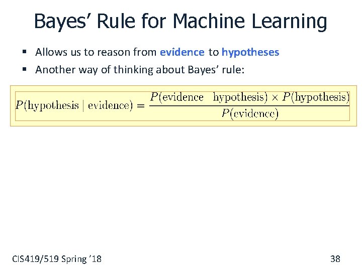
Bayes’ Rule for Machine Learning § Allows us to reason from evidence to hypotheses § Another way of thinking about Bayes’ rule: CIS 419/519 Spring ’ 18 38

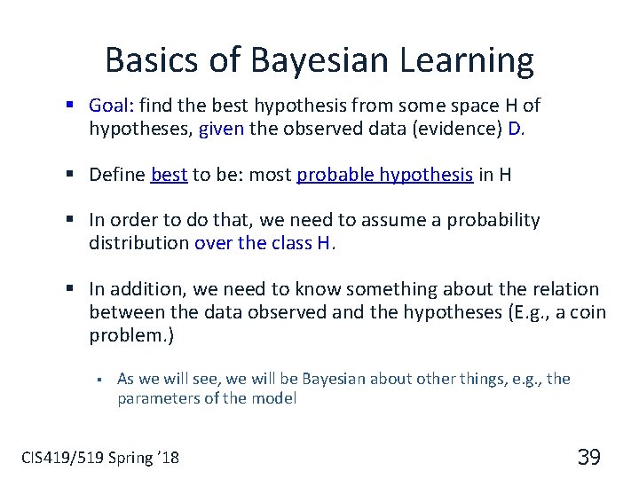
Basics of Bayesian Learning § Goal: find the best hypothesis from some space H of hypotheses, given the observed data (evidence) D. § Define best to be: most probable hypothesis in H § In order to do that, we need to assume a probability distribution over the class H. § In addition, we need to know something about the relation between the data observed and the hypotheses (E. g. , a coin problem. ) § As we will see, we will be Bayesian about other things, e. g. , the parameters of the model CIS 419/519 Spring ’ 18 39

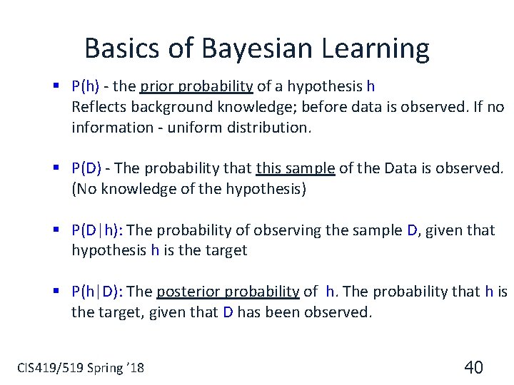
Basics of Bayesian Learning § P(h) - the prior probability of a hypothesis h Reflects background knowledge; before data is observed. If no information - uniform distribution. § P(D) - The probability that this sample of the Data is observed. (No knowledge of the hypothesis) § P(D|h): The probability of observing the sample D, given that hypothesis h is the target § P(h|D): The posterior probability of h. The probability that h is the target, given that D has been observed. CIS 419/519 Spring ’ 18 40

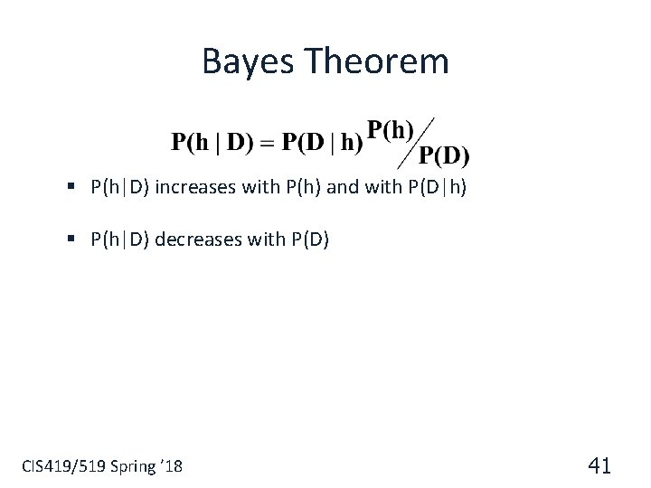
Bayes Theorem § P(h|D) increases with P(h) and with P(D|h) § P(h|D) decreases with P(D) CIS 419/519 Spring ’ 18 41

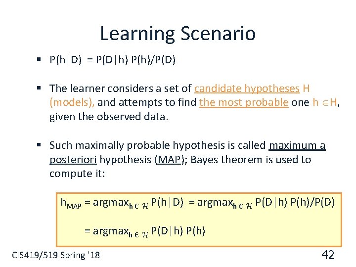
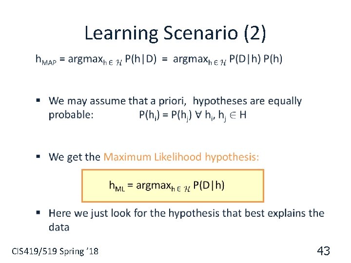
Learning Scenario § P(h|D) = P(D|h) P(h)/P(D) § The learner considers a set of candidate hypotheses H (models), and attempts to find the most probable one h H, given the observed data. § Such maximally probable hypothesis is called maximum a posteriori hypothesis (MAP); Bayes theorem is used to compute it: h. MAP = argmaxh Є H P(h|D) = argmaxh Є H P(D|h) P(h)/P(D) = argmaxh Є H P(D|h) P(h) CIS 419/519 Spring ’ 18 42

Learning Scenario (2) § CIS 419/519 Spring ’ 18 43

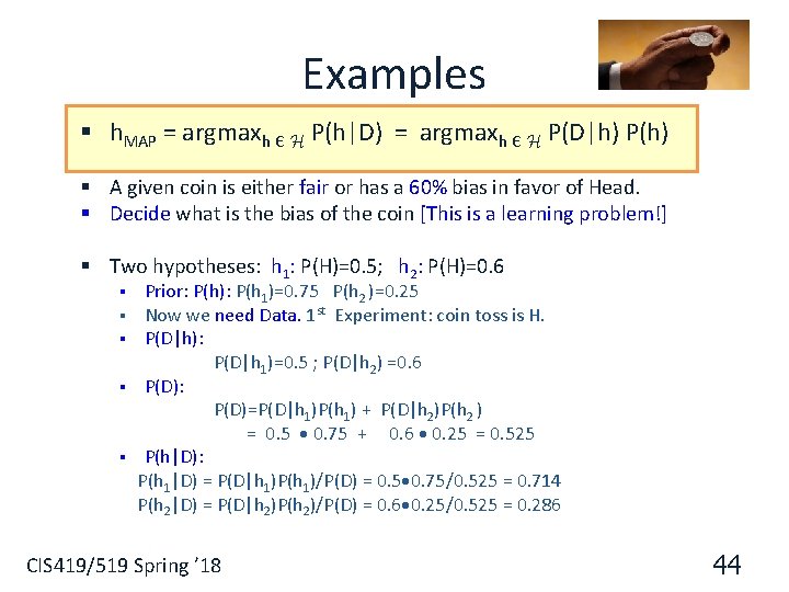
Examples § h. MAP = argmaxh Є H P(h|D) = argmaxh Є H P(D|h) P(h) § A given coin is either fair or has a 60% bias in favor of Head. § Decide what is the bias of the coin [This is a learning problem!] § Two hypotheses: h 1: P(H)=0. 5; h 2: P(H)=0. 6 § § § Prior: P(h): P(h 1)=0. 75 P(h 2 )=0. 25 Now we need Data. 1 st Experiment: coin toss is H. P(D|h): P(D|h 1)=0. 5 ; P(D|h 2) =0. 6 P(D): P(D)=P(D|h 1)P(h 1) + P(D|h 2)P(h 2 ) = 0. 5 0. 75 + 0. 6 0. 25 = 0. 525 P(h|D): P(h 1|D) = P(D|h 1)P(h 1)/P(D) = 0. 5 0. 75/0. 525 = 0. 714 P(h 2|D) = P(D|h 2)P(h 2)/P(D) = 0. 6 0. 25/0. 525 = 0. 286 CIS 419/519 Spring ’ 18 44

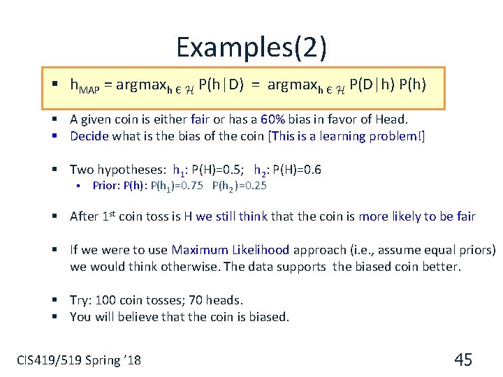
Examples(2) § h. MAP = argmaxh Є H P(h|D) = argmaxh Є H P(D|h) P(h) § A given coin is either fair or has a 60% bias in favor of Head. § Decide what is the bias of the coin [This is a learning problem!] § Two hypotheses: h 1: P(H)=0. 5; h 2: P(H)=0. 6 § Prior: P(h): P(h 1)=0. 75 P(h 2 )=0. 25 § After 1 st coin toss is H we still think that the coin is more likely to be fair § If we were to use Maximum Likelihood approach (i. e. , assume equal priors) we would think otherwise. The data supports the biased coin better. § Try: 100 coin tosses; 70 heads. § You will believe that the coin is biased. CIS 419/519 Spring ’ 18 45

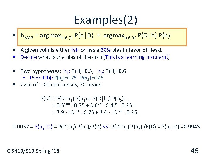
Examples(2) § h. MAP = argmaxh Є H P(h|D) = argmaxh Є H P(D|h) P(h) § A given coin is either fair or has a 60% bias in favor of Head. § Decide what is the bias of the coin [This is a learning problem!] § Two hypotheses: h 1: P(H)=0. 5; h 2: P(H)=0. 6 § Prior: P(h): P(h 1)=0. 75 P(h 2 )=0. 25 § Case of 100 coin tosses; 70 heads. P(D) = P(D|h 1) P(h 1) + P(D|h 2) P(h 2) = = 0. 5100 ¢ 0. 75 + 0. 670 ¢ 0. 430 ¢ 0. 25 = = 7. 9 ¢ 10 -31 ¢ 0. 75 + 3. 4 ¢ 10 -28 ¢ 0. 25 0. 0057 = P(h 1|D) = P(D|h 1) P(h 1)/P(D) << P(D|h 2) P(h 2) /P(D) = P(h 2|D) =0. 9943 CIS 419/519 Spring ’ 18 46

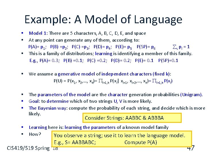
Example: A Model of Language Model 1: There are 5 characters, A, B, C, D, E, and space At any point can generate any of them, according to: P(A)= p 1; P(B) =p 2; P(C) =p 3; P(D)= p 4; P(E)= p 5 P(SP)= p 6 i pi = 1 § This is a family of distributions; learning is identifying a member of this family. E. g. , P(A)= 0. 3; P(B) =0. 1; P(C) =0. 2; P(D)= 0. 2; P(E)= 0. 1 P(SP)=0. 1 § § § We assume a generative model of independent characters (fixed k): P(U) = P(x 1, x 2, …, xk)= i=1, k P(xi| xi+1, xi+2, …, xk)= i=1, k P(xi) § § § The parameters of the model are the character generation probabilities (Unigram). Goal: to determine which of two strings U, V is more likely. The Bayesian way: compute the probability of each string, and decide which is more likely. Consider Strings: AABBC & ABBBA § § Learning here is: learning the parameters of a known model family How? You observe a string; use it to learn the language model. E. g. , S= AABBABC; CIS 419/519 Spring ’ 18 Compute P(A) 47

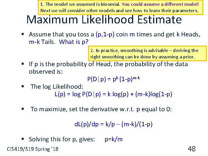
1. The model we assumed is binomial. You could assume a different model! Next we will consider other models and see how to learn their parameters. Maximum Likelihood Estimate § Assume that you toss a (p, 1 -p) coin m times and get k Heads, m-k Tails. What is p? 2. In practice, smoothing is advisable – deriving the right smoothing can be done by assuming a prior. § If p is the probability of Head, the probability of the data observed is: P(D|p) = pk (1 -p)m-k § The log Likelihood: L(p) = log P(D|p) = k log(p) + (m-k)log(1 -p) § To maximize, set the derivative w. r. t. p equal to 0: d. L(p)/dp = k/p – (m-k)/(1 -p) § Solving this for p, gives: CIS 419/519 Spring ’ 18 p=k/m 48

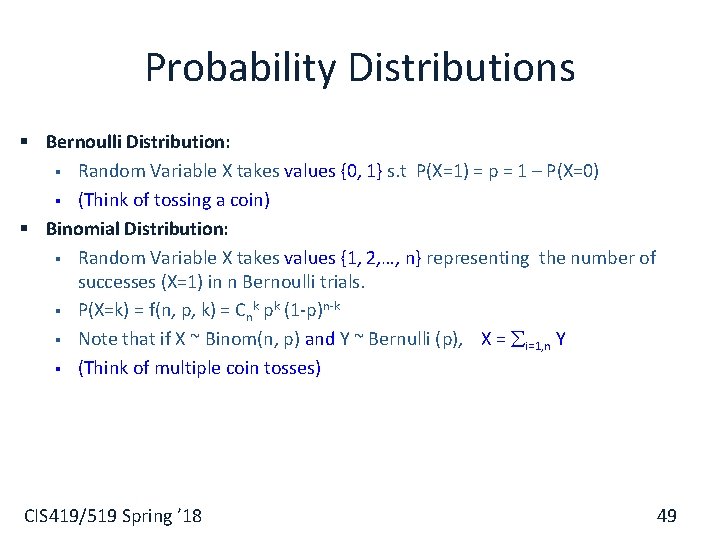
Probability Distributions § Bernoulli Distribution: § Random Variable X takes values {0, 1} s. t P(X=1) = p = 1 – P(X=0) § (Think of tossing a coin) § Binomial Distribution: § Random Variable X takes values {1, 2, …, n} representing the number of successes (X=1) in n Bernoulli trials. § P(X=k) = f(n, p, k) = Cnk pk (1 -p)n-k § Note that if X ~ Binom(n, p) and Y ~ Bernulli (p), X = i=1, n Y § (Think of multiple coin tosses) CIS 419/519 Spring ’ 18 49

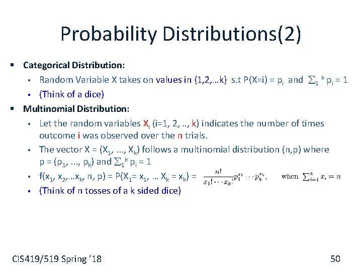
Probability Distributions(2) § Categorical Distribution: § Random Variable X takes on values in {1, 2, …k} s. t P(X=i) = pi and 1 k pi = 1 § (Think of a dice) § Multinomial Distribution: § Let the random variables Xi (i=1, 2, …, k) indicates the number of times outcome i was observed over the n trials. § The vector X = (X 1, . . . , Xk) follows a multinomial distribution (n, p) where p = (p 1, . . . , pk) and 1 k pi = 1 § f(x 1, x 2, …xk, n, p) = P(X 1= x 1, … Xk = xk) = § (Think of n tosses of a k sided dice) CIS 419/519 Spring ’ 18 50

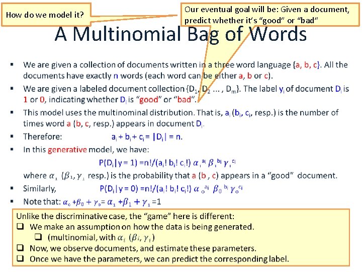
How do we model it? Our eventual goal will be: Given a document, predict whether it’s “good” or “bad” A Multinomial Bag of Words § CIS 419/519 Spring ’ 18 51

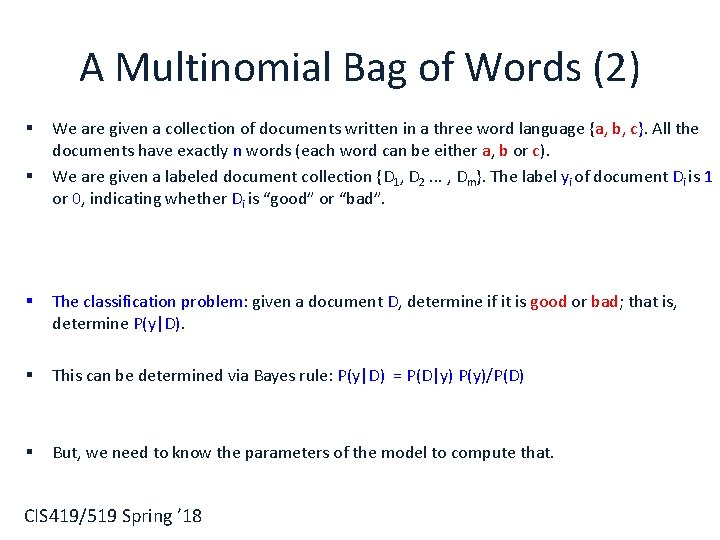
A Multinomial Bag of Words (2) § § We are given a collection of documents written in a three word language {a, b, c}. All the documents have exactly n words (each word can be either a, b or c). We are given a labeled document collection {D 1, D 2. . . , Dm}. The label yi of document Di is 1 or 0, indicating whether Di is “good” or “bad”. § The classification problem: given a document D, determine if it is good or bad; that is, determine P(y|D). § This can be determined via Bayes rule: P(y|D) = P(D|y) P(y)/P(D) § But, we need to know the parameters of the model to compute that. CIS 419/519 Spring ’ 18

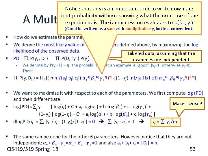
Notice that this is an important trick to write down the joint probability without knowing what the outcome of the experiment is. The ith expression evaluates to p(Di , yi) A Multinomial Bag of Words (3) (Could be written as a sum with multiplicative yi but less convenient) § Labeled data, assuming that the examples are independent Makes sense? CIS 419/519 Spring ’ 18 53

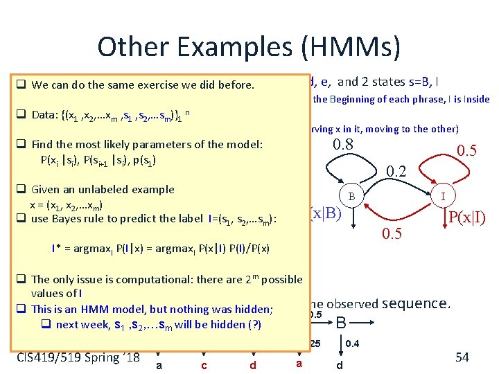
Other Examples (HMMs) data over 5 we characters, q We §can Consider do the same exercise did before. x=a, b, c, d, e, and 2 states s=B, I Think about chunking a sentence to phrases; B is the Beginning of each phrase, I is Inside n phrase. q Data: {(x 1 , x 2 a, …x m , s 1 , s 2, …sm)}1 § (Or: think about being in one of two rooms, observing x in it, moving to the other) § 0. 8 q Find§the. We most likely parameters of the model: to: generate characters according P(xi |si), P(si+1 |si), p(s 1) § Initial state prob: p(B)= 1; p(I)=0 P(B)=1 P(I) = 0 § an. State transition prob: q Given unlabeled example x = (x 1, x 2, …x § p(B B)=0. 8 p(B I)=0. 2 m) q use Bayes§ rule to predictp(I I)=0. 5 the label l=(s 1, s 2, …sm): p(I B)=0. 5 0. 2 B I P(x|B) 0. 5 §l* =Output argmaxlprob: P(l|x) = argmaxl P(x|l) P(l)/P(x) P(x|I) p(a|B) = 0. 25, p(b|B)=0. 10, p(c|B)=0. 10, …. q The only §issue is computational: there are 2 m possible p(a|I) = 0. 25, p(b, I)=0, … values of l follow thebut generation process to get the observed sequence. q This§is an. Can HMM model, nothing was 0. 2 0. 5 hidden; 0. 5 1 q next week, s 1 , s 2, …s B m will be. I hidden (? ) I I B § CIS 419/519 Spring ’ 18 0. 25 a 0. 25 c 0. 25 d 0. 25 a 0. 4 d 54

Bayes Optimal Classifier § How should we use the general formalism? § What should H be? § H can be a collection of functions. Given the training data, choose an optimal function. Then, given new data, evaluate the selected function on it. § H can be a collection of possible predictions. Given the data, try to directly choose the optimal prediction. § Could be different! CIS 419/519 Spring ’ 18 55

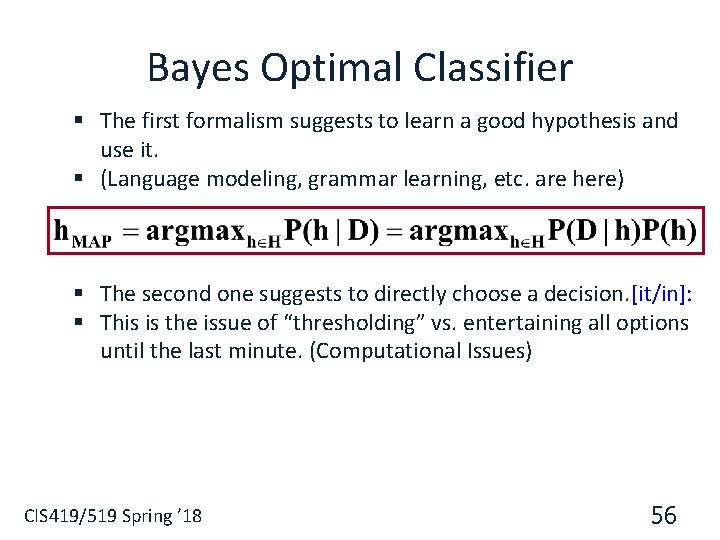
Bayes Optimal Classifier § The first formalism suggests to learn a good hypothesis and use it. § (Language modeling, grammar learning, etc. are here) § The second one suggests to directly choose a decision. [it/in]: § This is the issue of “thresholding” vs. entertaining all options until the last minute. (Computational Issues) CIS 419/519 Spring ’ 18 56

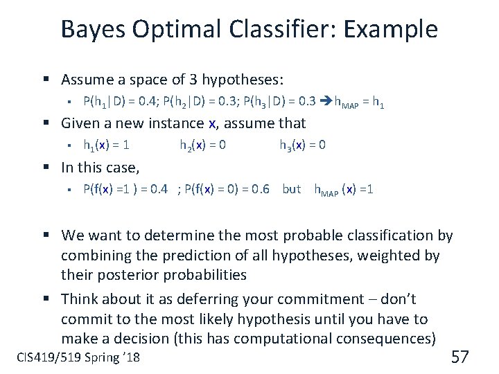
Bayes Optimal Classifier: Example § Assume a space of 3 hypotheses: § P(h 1|D) = 0. 4; P(h 2|D) = 0. 3; P(h 3|D) = 0. 3 h. MAP = h 1 § Given a new instance x, assume that § h 1(x) = 1 h 2(x) = 0 h 3(x) = 0 § In this case, § P(f(x) =1 ) = 0. 4 ; P(f(x) = 0. 6 but h. MAP (x) =1 § We want to determine the most probable classification by combining the prediction of all hypotheses, weighted by their posterior probabilities § Think about it as deferring your commitment – don’t commit to the most likely hypothesis until you have to make a decision (this has computational consequences) CIS 419/519 Spring ’ 18 57

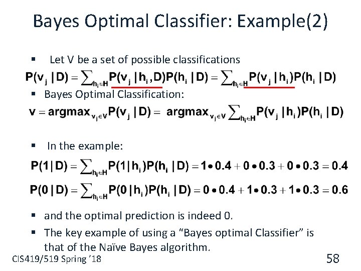
Bayes Optimal Classifier: Example(2) § Let V be a set of possible classifications § Bayes Optimal Classification: § In the example: § and the optimal prediction is indeed 0. § The key example of using a “Bayes optimal Classifier” is that of the Naïve Bayes algorithm. CIS 419/519 Spring ’ 18 58

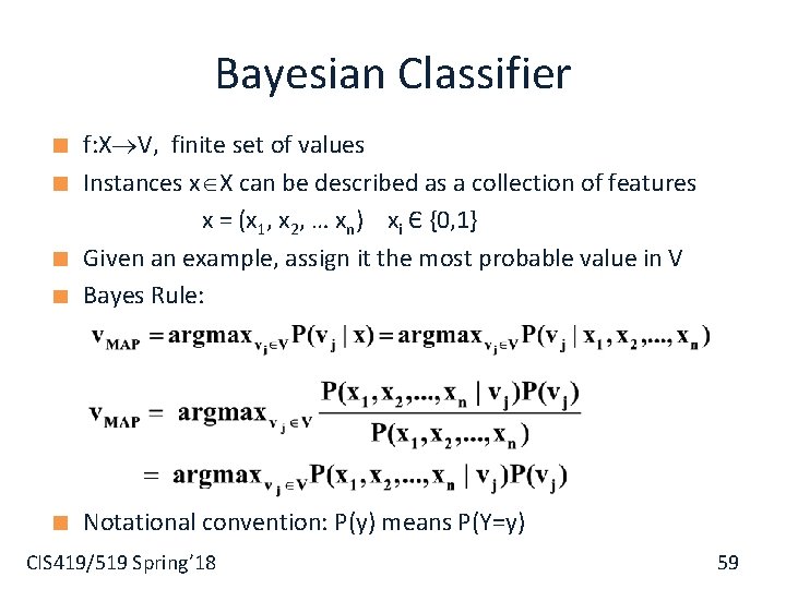
Bayesian Classifier f: X V, finite set of values Instances x X can be described as a collection of features x = (x 1, x 2, … xn) xi Є {0, 1} Given an example, assign it the most probable value in V Bayes Rule: Notational convention: P(y) means P(Y=y) CIS 419/519 Spring’ 18 59

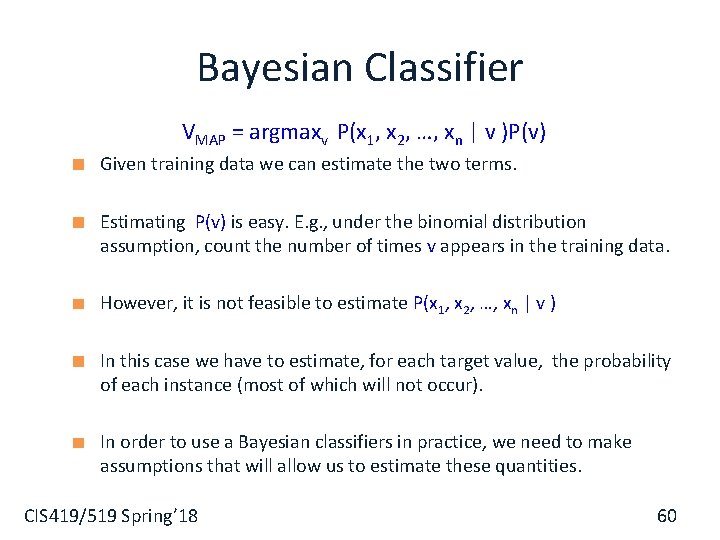
Bayesian Classifier VMAP = argmaxv P(x 1, x 2, …, xn | v )P(v) Given training data we can estimate the two terms. Estimating P(v) is easy. E. g. , under the binomial distribution assumption, count the number of times v appears in the training data. However, it is not feasible to estimate P(x 1, x 2, …, xn | v ) In this case we have to estimate, for each target value, the probability of each instance (most of which will not occur). In order to use a Bayesian classifiers in practice, we need to make assumptions that will allow us to estimate these quantities. CIS 419/519 Spring’ 18 60

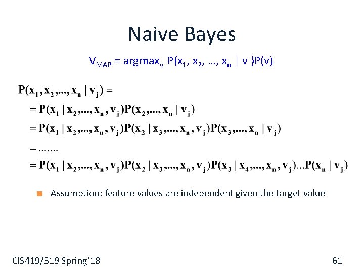
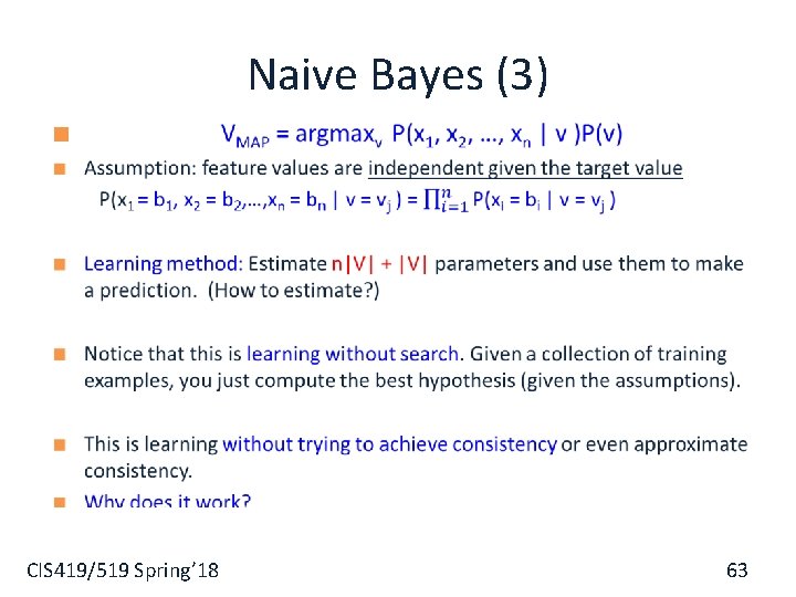
Naive Bayes VMAP = argmaxv P(x 1, x 2, …, xn | v )P(v) Assumption: feature values are independent given the target value CIS 419/519 Spring’ 18 61

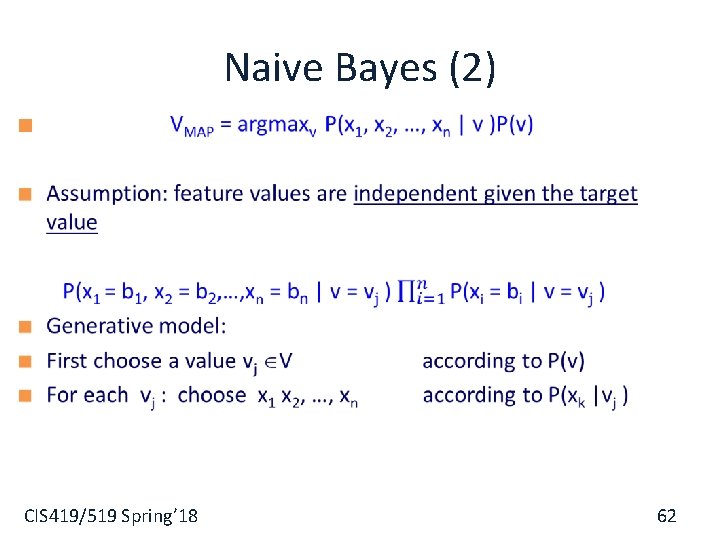
Naive Bayes (2) CIS 419/519 Spring’ 18 62

Naive Bayes (3) CIS 419/519 Spring’ 18 63

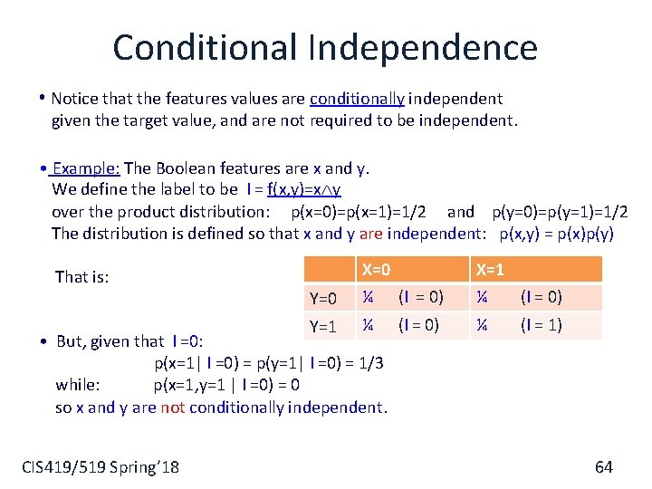
Conditional Independence • Notice that the features values are conditionally independent given the target value, and are not required to be independent. • Example: The Boolean features are x and y. We define the label to be l = f(x, y)=x y over the product distribution: p(x=0)=p(x=1)=1/2 and p(y=0)=p(y=1)=1/2 The distribution is defined so that x and y are independent: p(x, y) = p(x)p(y) That is: Y=0 X=0 ¼ (l = 0) X=1 ¼ (l = 0) Y=1 ¼ ¼ • But, given that l =0: p(x=1| l =0) = p(y=1| l =0) = 1/3 while: p(x=1, y=1 | l =0) = 0 so x and y are not conditionally independent. CIS 419/519 Spring’ 18 (l = 0) (l = 1) 64

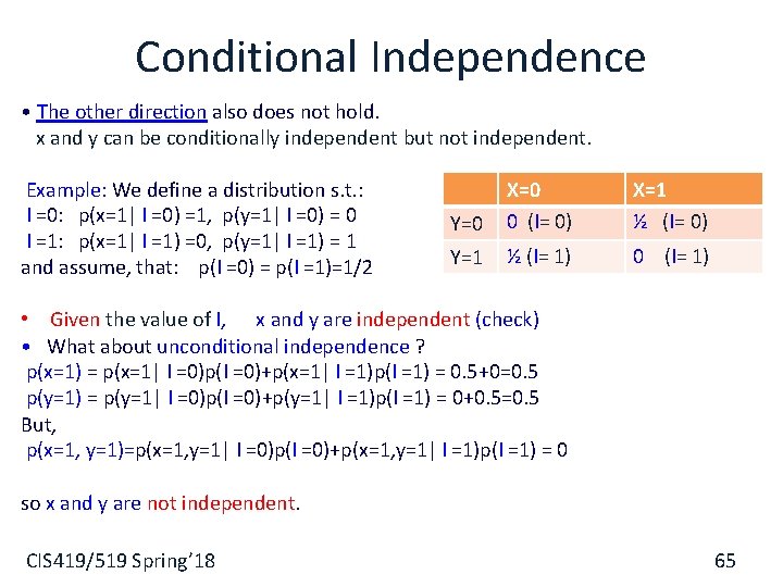
Conditional Independence • The other direction also does not hold. x and y can be conditionally independent but not independent. Example: We define a distribution s. t. : l =0: p(x=1| l =0) =1, p(y=1| l =0) = 0 l =1: p(x=1| l =1) =0, p(y=1| l =1) = 1 and assume, that: p(l =0) = p(l =1)=1/2 Y=0 X=0 0 (l= 0) X=1 ½ (l= 0) Y=1 ½ (l= 1) 0 (l= 1) • Given the value of l, x and y are independent (check) • What about unconditional independence ? p(x=1) = p(x=1| l =0)p(l =0)+p(x=1| l =1)p(l =1) = 0. 5+0=0. 5 p(y=1) = p(y=1| l =0)p(l =0)+p(y=1| l =1)p(l =1) = 0+0. 5=0. 5 But, p(x=1, y=1)=p(x=1, y=1| l =0)p(l =0)+p(x=1, y=1| l =1)p(l =1) = 0 so x and y are not independent. CIS 419/519 Spring’ 18 65

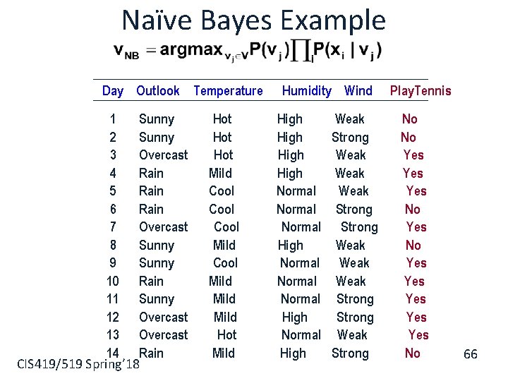
Naïve Bayes Example Day Outlook Temperature 1 Sunny 2 Sunny 3 Overcast 4 Rain 5 Rain 6 Rain 7 Overcast 8 Sunny 9 Sunny 10 Rain 11 Sunny 12 Overcast 13 Overcast 14 Rain CIS 419/519 Spring’ 18 Hot Hot Mild Cool Mild Hot Mild Humidity Wind High Normal Normal High Weak Strong Weak Weak Strong Weak Strong Play. Tennis No No Yes Yes Yes No 66

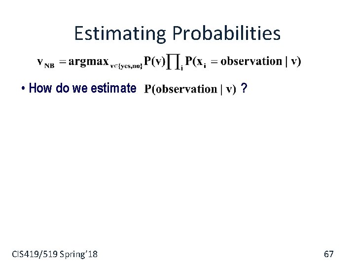
Estimating Probabilities • How do we estimate CIS 419/519 Spring’ 18 ? 67

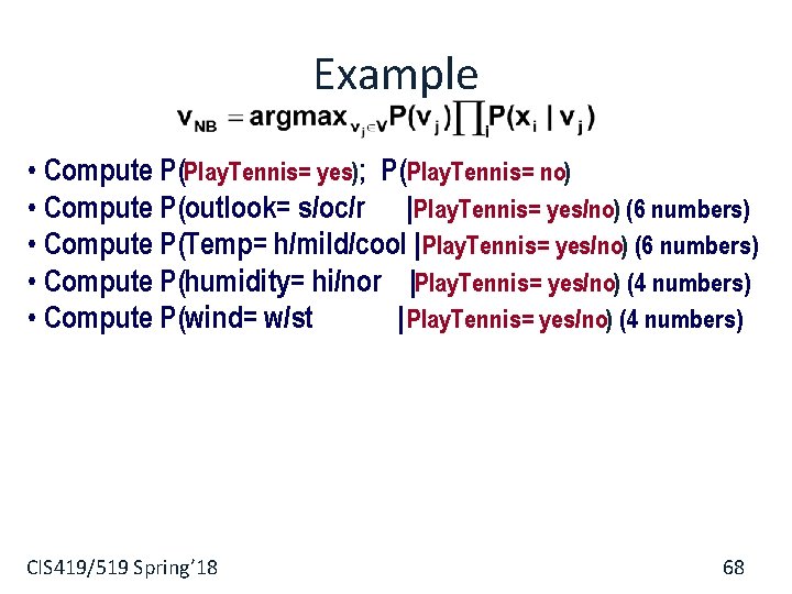
Example • Compute P(Play. Tennis= yes); P(Play. Tennis= no) • Compute P(outlook= s/oc/r |Play. Tennis= yes/no) (6 numbers) • Compute P(Temp= h/mild/cool |Play. Tennis= yes/no) (6 numbers) • Compute P(humidity= hi/nor |Play. Tennis= yes/no) (4 numbers) • Compute P(wind= w/st | Play. Tennis= yes/no) (4 numbers) CIS 419/519 Spring’ 18 68

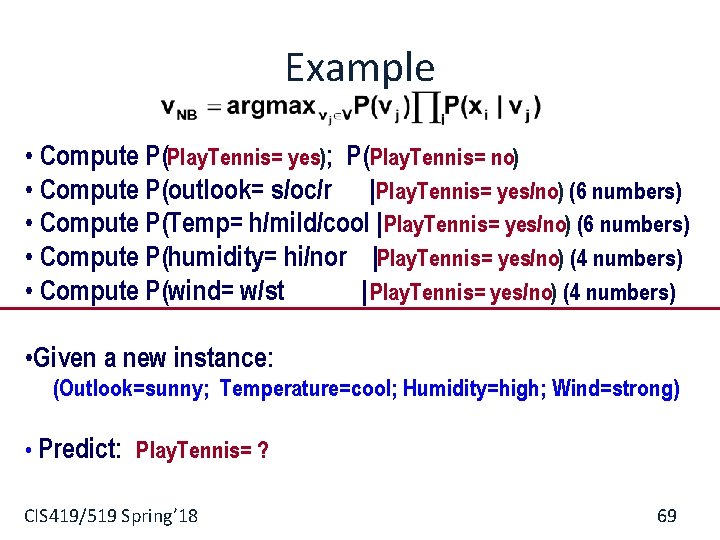
Example • Compute P(Play. Tennis= yes); P(Play. Tennis= no) • Compute P(outlook= s/oc/r |Play. Tennis= yes/no) (6 numbers) • Compute P(Temp= h/mild/cool |Play. Tennis= yes/no) (6 numbers) • Compute P(humidity= hi/nor |Play. Tennis= yes/no) (4 numbers) • Compute P(wind= w/st | Play. Tennis= yes/no) (4 numbers) • Given a new instance: (Outlook=sunny; Temperature=cool; Humidity=high; Wind=strong) • Predict: Play. Tennis= ? CIS 419/519 Spring’ 18 69

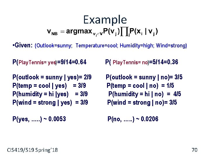
Example • Given: (Outlook=sunny; Temperature=cool; Humidity=high; Wind=strong) P( Play. Tennis= yes)=9/14=0. 64 P( Play. Tennis= no)=5/14=0. 36 P(outlook = sunny | yes)= 2/9 P(temp = cool | yes) = 3/9 P(humidity = hi |yes) = 3/9 P(wind = strong | yes) = 3/9 P(outlook = sunny | no)= 3/5 P(temp = cool | no) = 1/5 P(humidity = hi | no) = 4/5 P(wind = strong | no)= 3/5 P(yes, …. . ) ~ 0. 0053 P(no, …. . ) ~ 0. 0206 CIS 419/519 Spring’ 18 70

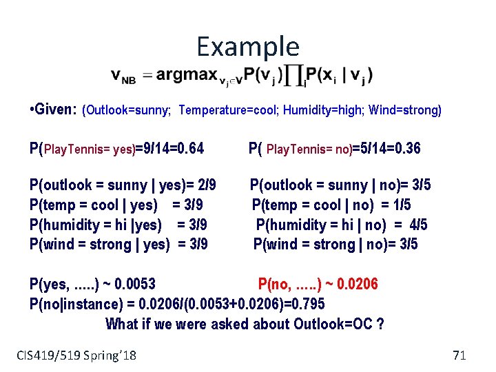
Example • Given: (Outlook=sunny; Temperature=cool; Humidity=high; Wind=strong) P( Play. Tennis= yes)=9/14=0. 64 P( Play. Tennis= no)=5/14=0. 36 P(outlook = sunny | yes)= 2/9 P(temp = cool | yes) = 3/9 P(humidity = hi |yes) = 3/9 P(wind = strong | yes) = 3/9 P(outlook = sunny | no)= 3/5 P(temp = cool | no) = 1/5 P(humidity = hi | no) = 4/5 P(wind = strong | no)= 3/5 P(yes, …. . ) ~ 0. 0053 P(no, …. . ) ~ 0. 0206 P(no|instance) = 0. 0206/(0. 0053+0. 0206)=0. 795 What if we were asked about Outlook=OC ? CIS 419/519 Spring’ 18 71

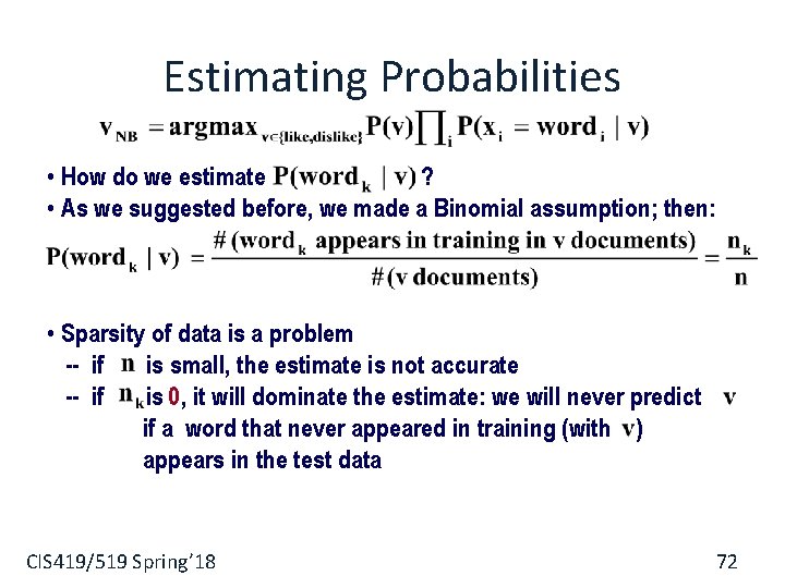
Estimating Probabilities • How do we estimate ? • As we suggested before, we made a Binomial assumption; then: • Sparsity of data is a problem -- if is small, the estimate is not accurate -- if is 0, it will dominate the estimate: we will never predict if a word that never appeared in training (with ) appears in the test data CIS 419/519 Spring’ 18 72

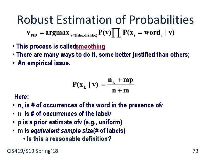
Robust Estimation of Probabilities • This process is calledsmoothing. • There are many ways to do it, some better justified than others; • An empirical issue. Here: • nk is # of occurrences of the word in the presence ofv • n is # of occurrences of the labelv • p is a prior estimate ofv (e. g. , uniform) • m is equivalent sample size (# of labels) • Is this a reasonable definition? CIS 419/519 Spring’ 18 73

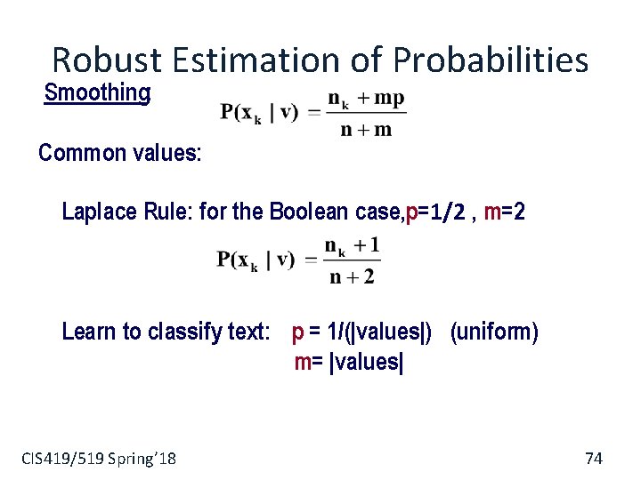
Robust Estimation of Probabilities Smoothing: Common values: Laplace Rule: for the Boolean case, p=1/2 , m=2 Learn to classify text: p = 1/(|values|) (uniform) m= |values| CIS 419/519 Spring’ 18 74

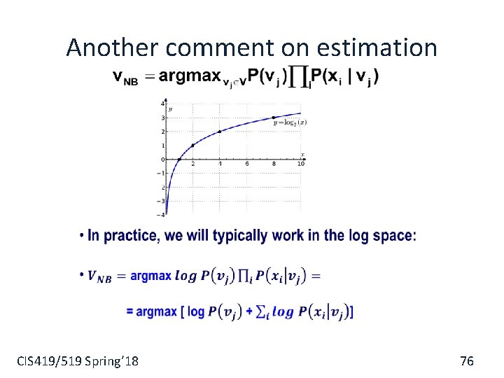
Another comment on estimation CIS 419/519 Spring’ 18 76

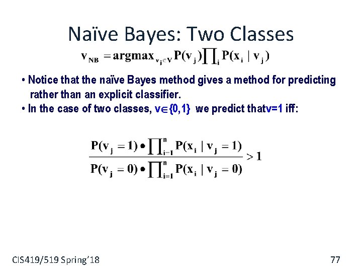
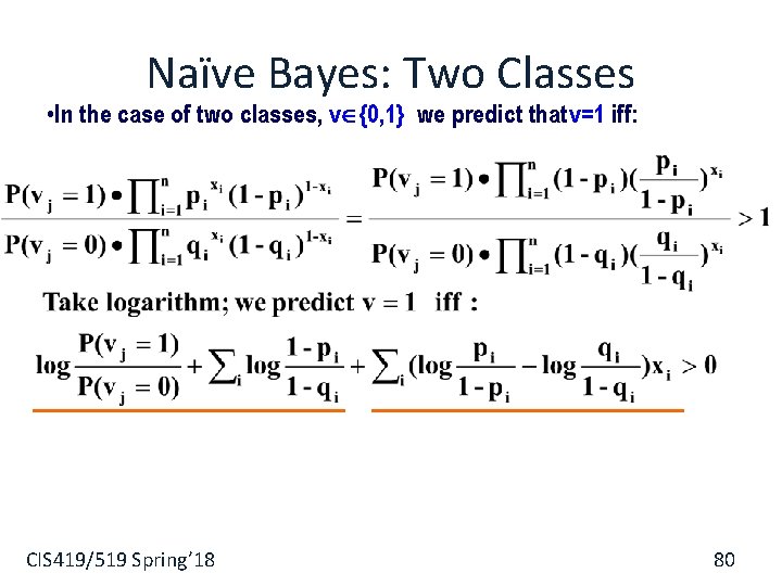
Naïve Bayes: Two Classes • Notice that the naïve Bayes method gives a method for predicting rather than an explicit classifier. • In the case of two classes, v {0, 1} we predict that v=1 iff: CIS 419/519 Spring’ 18 77

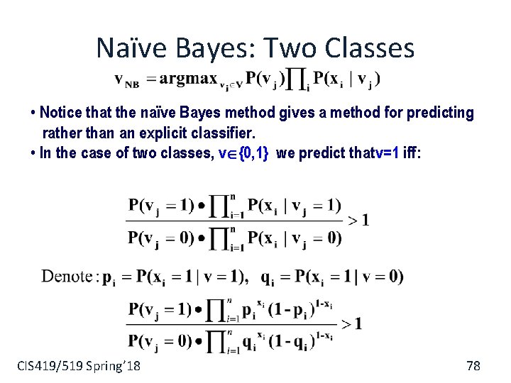
Naïve Bayes: Two Classes • Notice that the naïve Bayes method gives a method for predicting rather than an explicit classifier. • In the case of two classes, v {0, 1} we predict that v=1 iff: CIS 419/519 Spring’ 18 78

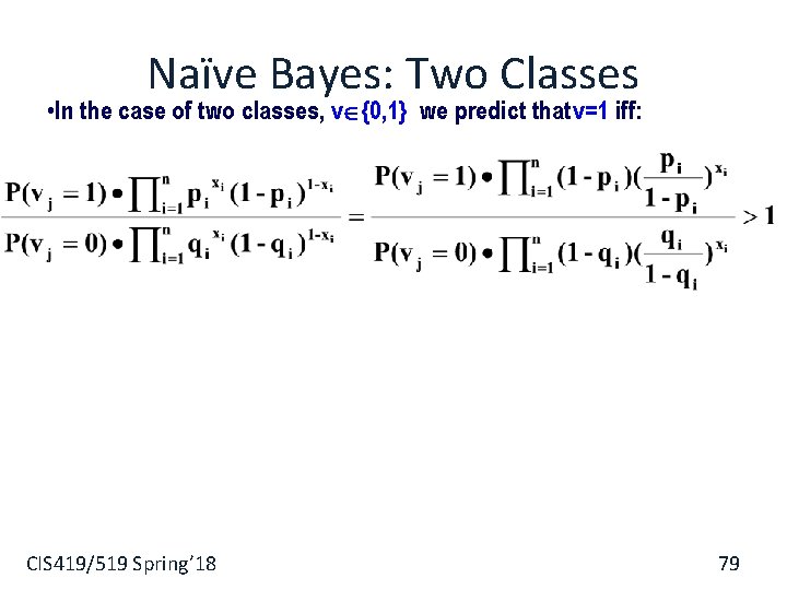
Naïve Bayes: Two Classes • In the case of two classes, v {0, 1} we predict that v=1 iff: CIS 419/519 Spring’ 18 79

Naïve Bayes: Two Classes • In the case of two classes, v {0, 1} we predict that v=1 iff: CIS 419/519 Spring’ 18 80

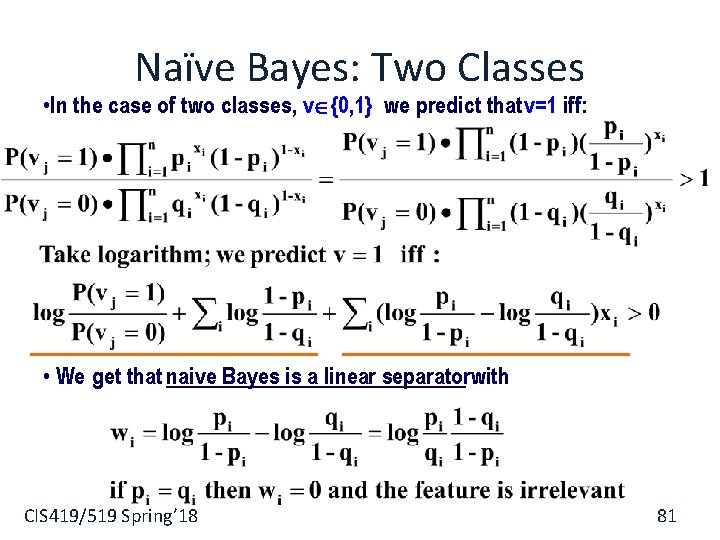
Naïve Bayes: Two Classes • In the case of two classes, v {0, 1} we predict that v=1 iff: • We get that naive Bayes is a linear separatorwith CIS 419/519 Spring’ 18 81

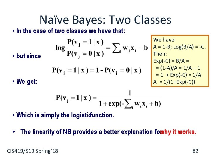
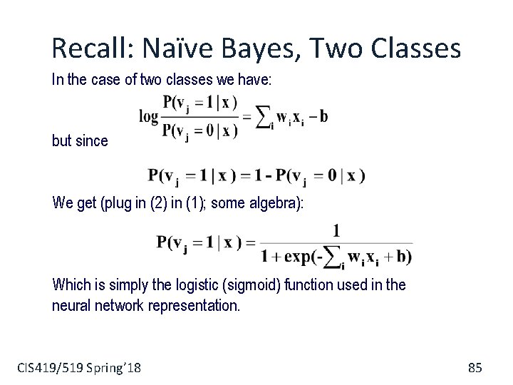
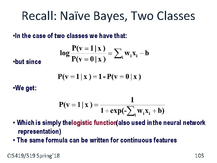
Naïve Bayes: Two Classes • In the case of two classes we have that: • but since • We get: We have: A = 1 -B; Log(B/A) = -C. Then: Exp(-C) = B/A = = (1 -A)/A = 1/A – 1 = 1 + Exp(-C) = 1/A A = 1/(1+Exp(-C)) • Which is simply the logisticfunction. • The linearity of NB provides a better explanation forwhy it works. CIS 419/519 Spring’ 18 82

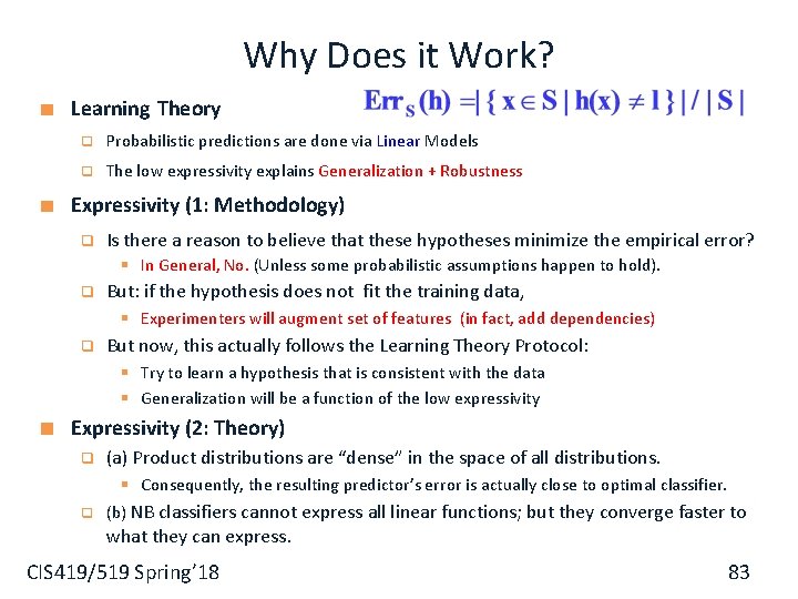
Why Does it Work? Learning Theory q Probabilistic predictions are done via Linear Models q The low expressivity explains Generalization + Robustness Expressivity (1: Methodology) q Is there a reason to believe that these hypotheses minimize the empirical error? § In General, No. (Unless some probabilistic assumptions happen to hold). q But: if the hypothesis does not fit the training data, § Experimenters will augment set of features (in fact, add dependencies) q But now, this actually follows the Learning Theory Protocol: § Try to learn a hypothesis that is consistent with the data § Generalization will be a function of the low expressivity Expressivity (2: Theory) q (a) Product distributions are “dense” in the space of all distributions. § Consequently, the resulting predictor’s error is actually close to optimal classifier. q (b) NB classifiers cannot express all linear functions; but they converge faster to what they can express. CIS 419/519 Spring’ 18 83

What’s Next? (1) If probabilistic hypotheses are actually like other linear functions, can we interpret the outcome of other linear learning algorithms probabilistically? q Yes (2) If probabilistic hypotheses are actually like other linear functions, can you train them similarly (that is, discriminatively)? q q q Yes. Classification: Logistics regression/Max Entropy HMM: can be learned as a linear model, e. g. , with a version of Perceptron (Structured Models class) CIS 419/519 Spring’ 18 84

Recall: Naïve Bayes, Two Classes In the case of two classes we have: but since We get (plug in (2) in (1); some algebra): Which is simply the logistic (sigmoid) function used in the neural network representation. CIS 419/519 Spring’ 18 85

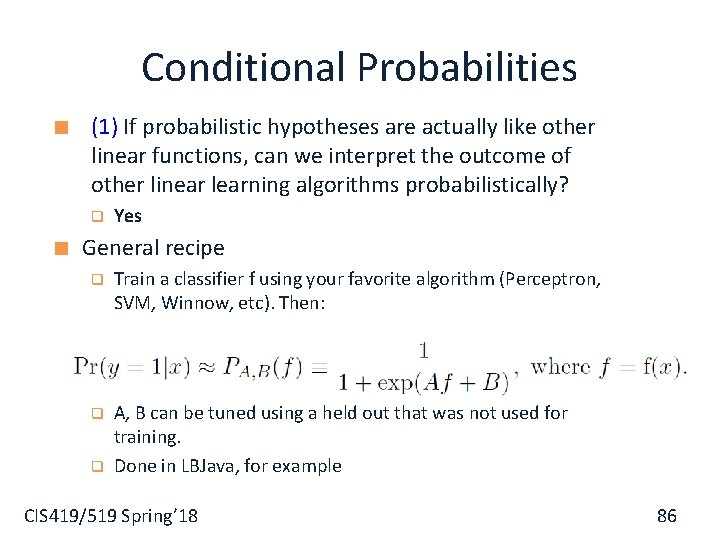
Conditional Probabilities (1) If probabilistic hypotheses are actually like other linear functions, can we interpret the outcome of other linear learning algorithms probabilistically? q Yes General recipe q Train a classifier f using your favorite algorithm (Perceptron, SVM, Winnow, etc). Then: q Use Sigmoid 1/1+exp{-(Aw. Tx + B)} to get an estimate for P(y | x) A, B can be tuned using a held out that was not used for training. Done in LBJava, for example q q CIS 419/519 Spring’ 18 86

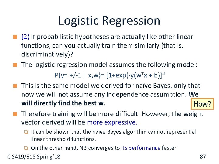
Logistic Regression (2) If probabilistic hypotheses are actually like other linear functions, can you actually train them similarly (that is, discriminatively)? The logistic regression model assumes the following model: P(y= +/-1 | x, w)= [1+exp(-y(w. Tx + b)]-1 This is the same model we derived for naïve Bayes, only that now we will not assume any independence assumption. We will directly find the best w. How? Therefore training will be more difficult. However, the weight vector derived will be more expressive. It can be shown that the naïve Bayes algorithm cannot represent all linear threshold functions. q On the other hand, NB converges to its performance faster. 87 CIS 419/519 Spring’ 18 q

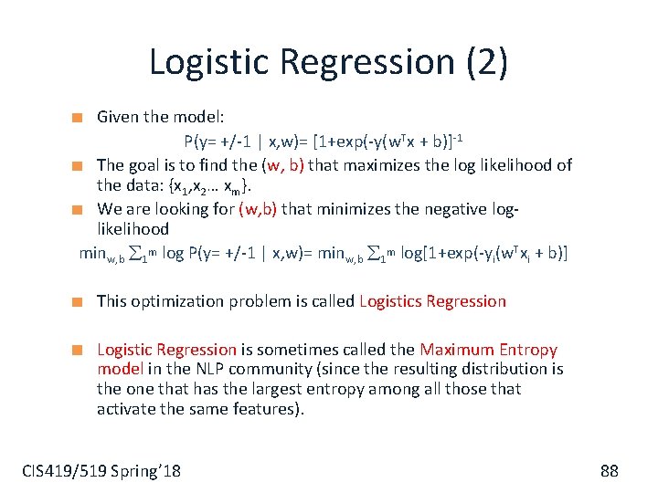
Logistic Regression (2) Given the model: P(y= +/-1 | x, w)= [1+exp(-y(w. Tx + b)]-1 The goal is to find the (w, b) that maximizes the log likelihood of the data: {x 1, x 2… xm}. We are looking for (w, b) that minimizes the negative loglikelihood minw, b 1 m log P(y= +/-1 | x, w)= minw, b 1 m log[1+exp(-yi(w. Txi + b)] This optimization problem is called Logistics Regression Logistic Regression is sometimes called the Maximum Entropy model in the NLP community (since the resulting distribution is the one that has the largest entropy among all those that activate the same features). CIS 419/519 Spring’ 18 88

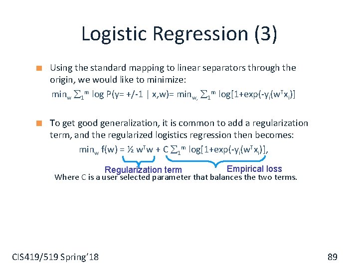
Logistic Regression (3) Using the standard mapping to linear separators through the origin, we would like to minimize: minw 1 m log P(y= +/-1 | x, w)= minw, 1 m log[1+exp(-yi(w. Txi)] To get good generalization, it is common to add a regularization term, and the regularized logistics regression then becomes: minw f(w) = ½ w. Tw + C 1 m log[1+exp(-yi(w. Txi)], Empirical loss Regularization term Where C is a user selected parameter that balances the two terms. CIS 419/519 Spring’ 18 89

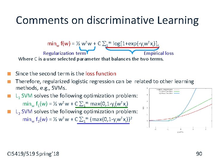
Comments on discriminative Learning minw f(w) = ½ w. Tw + C 1 m log[1+exp(-yiw. Txi)], Regularization term Empirical loss Where C is a user selected parameter that balances the two terms. Since the second term is the loss function Therefore, regularized logistic regression can be related to other learning methods, e. g. , SVMs. L 1 SVM solves the following optimization problem: minw f 1(w) = ½ w. Tw + C 1 m max(0, 1 -yi(w. Txi) L 2 SVM solves the following optimization problem: minw f 2(w) = ½ w. Tw + C 1 m (max(0, 1 -yiw. Txi))2 CIS 419/519 Spring’ 18 90

A few more NB examples CIS 419/519 Spring’ 18 91

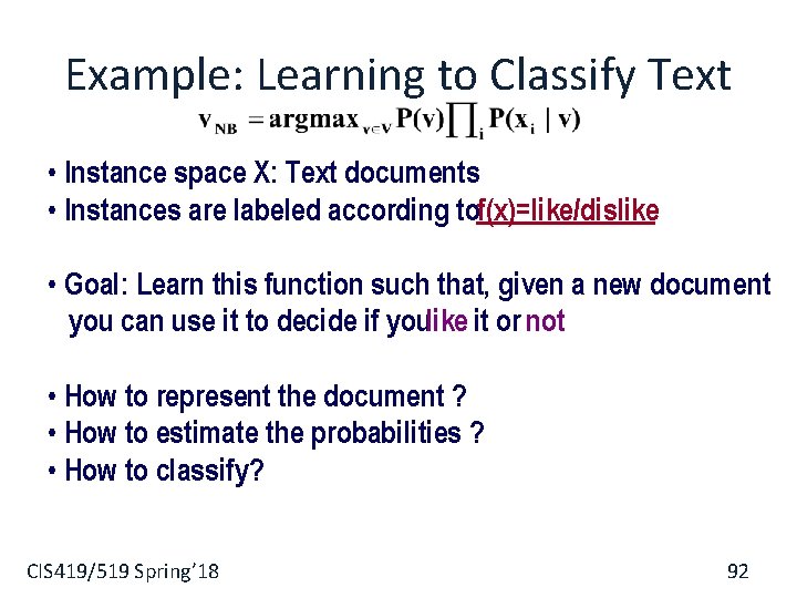
Example: Learning to Classify Text • Instance space X: Text documents • Instances are labeled according tof(x)=like/dislike • Goal: Learn this function such that, given a new document you can use it to decide if youlike it or not • How to represent the document ? • How to estimate the probabilities ? • How to classify? CIS 419/519 Spring’ 18 92

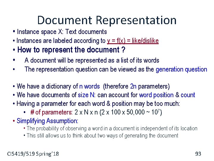
Document Representation • Instance space X: Text documents • Instances are labeled according to y = f(x) = like/dislike • How to represent the document ? • A document will be represented as a list of its words • The representation question can be viewed as the generation question • We have a dictionary of n words (therefore 2 n parameters) • We have documents of size N: can account for word position & count • Having a parameter for each word & position may be too much: • # of parameters: 2 x N x n (2 x 100 x 50, 000 ~ 107) • Simplifying Assumption: • The probability of observing a word in a document is independent of its location • This still allows us to think about two ways of generating the document CIS 419/519 Spring’ 18 93

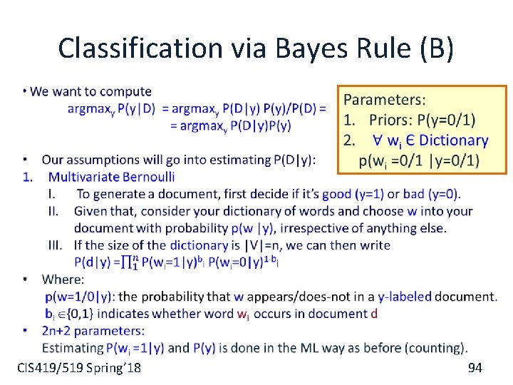
Classification via Bayes Rule (B) CIS 419/519 Spring’ 18 94

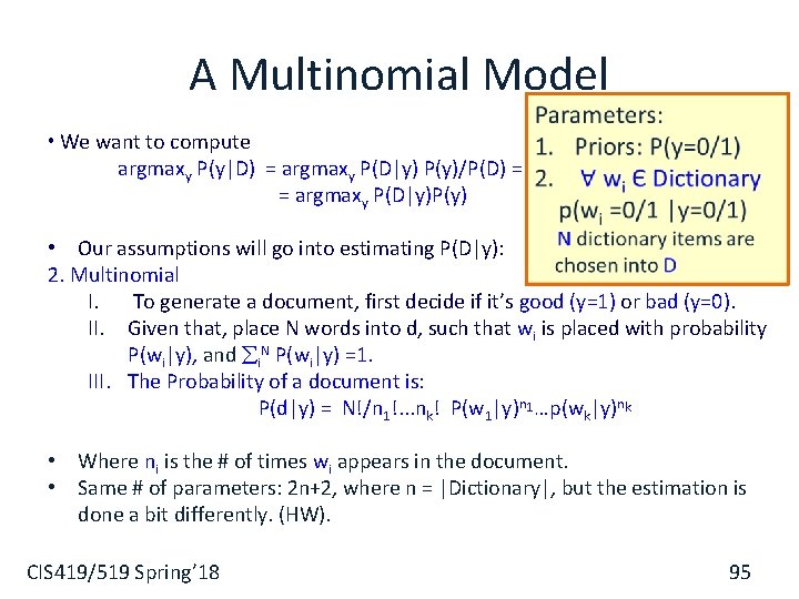
A Multinomial Model • We want to compute argmaxy P(y|D) = argmaxy P(D|y) P(y)/P(D) = = argmaxy P(D|y)P(y) • Our assumptions will go into estimating P(D|y): 2. Multinomial I. To generate a document, first decide if it’s good (y=1) or bad (y=0). II. Given that, place N words into d, such that wi is placed with probability P(wi|y), and i. N P(wi|y) =1. III. The Probability of a document is: P(d|y) = N!/n 1!. . . nk! P(w 1|y)n 1…p(wk|y)nk • Where ni is the # of times wi appears in the document. • Same # of parameters: 2 n+2, where n = |Dictionary|, but the estimation is done a bit differently. (HW). CIS 419/519 Spring’ 18 95

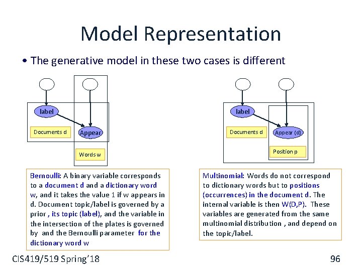
Model Representation • The generative model in these two cases is different label Documents d label Appear Words w Bernoulli: A binary variable corresponds to a document d and a dictionary word w, and it takes the value 1 if w appears in d. Document topic/label is governed by a prior , its topic (label), and the variable in the intersection of the plates is governed by and the Bernoulli parameter for the dictionary word w CIS 419/519 Spring’ 18 Documents d Appear (d) Position p Multinomial: Words do not correspond to dictionary words but to positions (occurrences) in the document d. The internal variable is then W(D, P). These variables are generated from the same multinomial distribution , and depend on the topic/label. 96

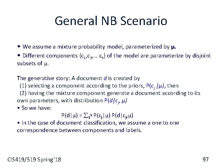
General NB Scenario • We assume a mixture probability model, parameterized by µ. • Different components {c 1, c 2, … ck} of the model are parameterize by disjoint subsets of µ. The generative story: A document d is created by (1) selecting a component according to the priors, P(cj |µ), then (2) having the mixture component generate a document according to its own parameters, with distribution P(d|cj, µ) • So we have: P(d|µ) = 1 k P(cj|µ) P(d|cj, µ) • In the case of document classification, we assume a one to one correspondence between components and labels. CIS 419/519 Spring’ 18 97

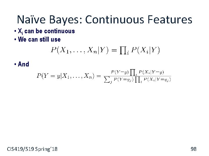
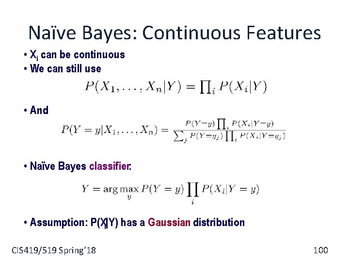
Naïve Bayes: Continuous Features • Xi can be continuous • We can still use • And CIS 419/519 Spring’ 18 98

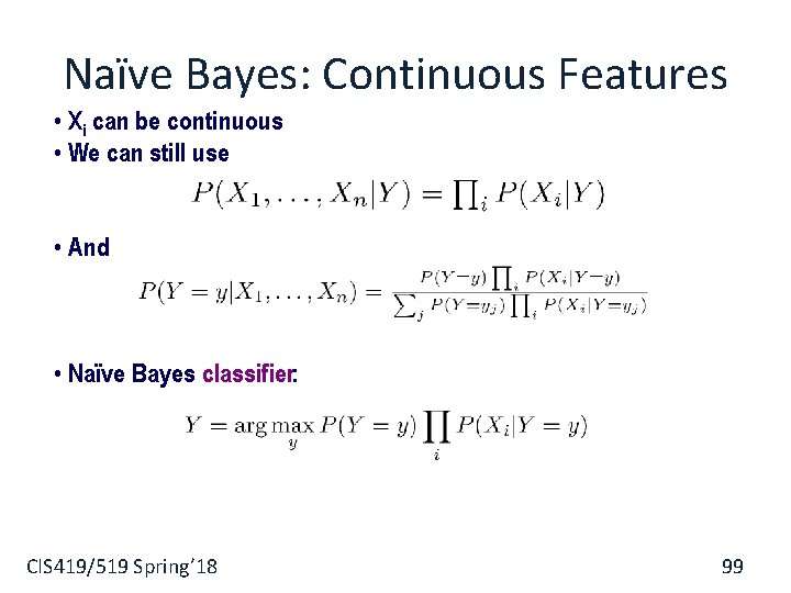
Naïve Bayes: Continuous Features • Xi can be continuous • We can still use • And • Naïve Bayes classifier: CIS 419/519 Spring’ 18 99

Naïve Bayes: Continuous Features • Xi can be continuous • We can still use • And • Naïve Bayes classifier: • Assumption: P(Xi|Y) has a Gaussian distribution CIS 419/519 Spring’ 18 100

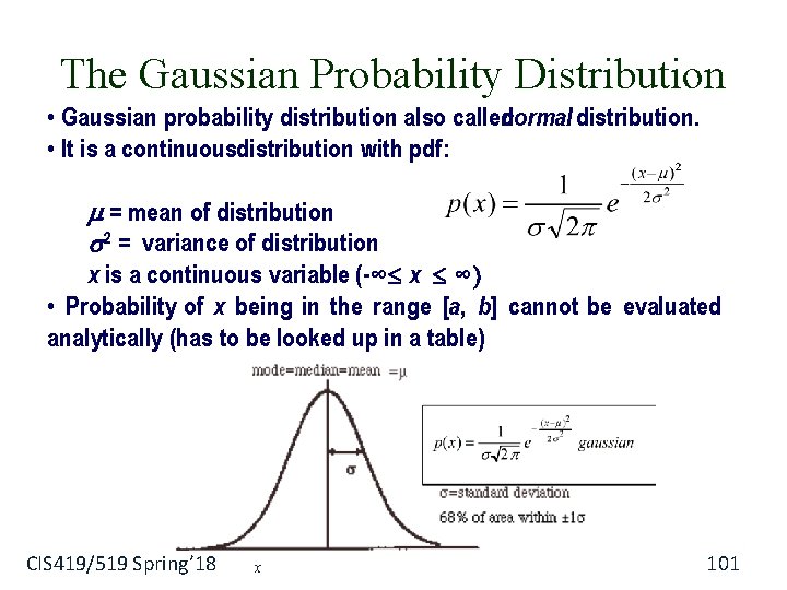
The Gaussian Probability Distribution • Gaussian probability distribution also callednormal distribution. • It is a continuousdistribution with pdf: = mean of distribution 2 = variance of distribution x is a continuous variable (-∞ x ∞ • Probability of x being in the range [a, b] cannot be evaluated analytically (has to be looked up in a table) CIS 419/519 Spring’ 18 x 101

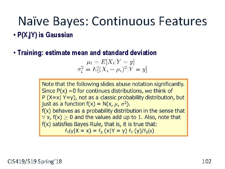
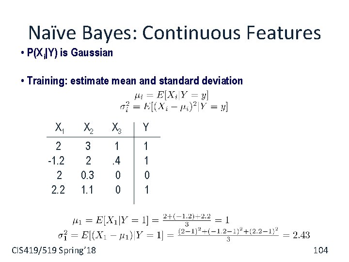
Naïve Bayes: Continuous Features • P(X i|Y) is Gaussian • Training: estimate mean and standard deviation CIS 419/519 Spring’ 18 102

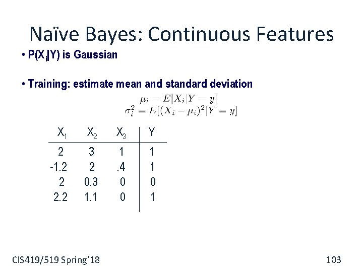
Naïve Bayes: Continuous Features • P(X i|Y) is Gaussian • Training: estimate mean and standard deviation X 1 X 2 X 3 Y 2 -1. 2 2 2. 2 3 2 0. 3 1. 1 1. 4 0 0 1 1 0 1 CIS 419/519 Spring’ 18 103

Naïve Bayes: Continuous Features • P(X i|Y) is Gaussian • Training: estimate mean and standard deviation X 1 X 2 X 3 Y 2 -1. 2 2 2. 2 3 2 0. 3 1. 1 1. 4 0 0 1 1 0 1 CIS 419/519 Spring’ 18 104

Recall: Naïve Bayes, Two Classes • In the case of two classes we have that: • but since • We get: • Which is simply thelogistic function(also used in the neural network representation) • The same formula can be written for continuous features CIS 419/519 Spring’ 18 105

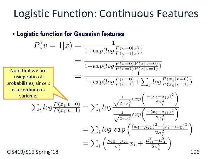
Logistic Function: Continuous Features • Logistic function for Gaussian features Note that we are using ratio of probabilities, since x is a continuous variable. CIS 419/519 Spring’ 18 106