Cholesky decomposition May 27 th 2015 Helsinki Finland

Cholesky decomposition May 27 th 2015 Helsinki, Finland E. Vuoksimaa

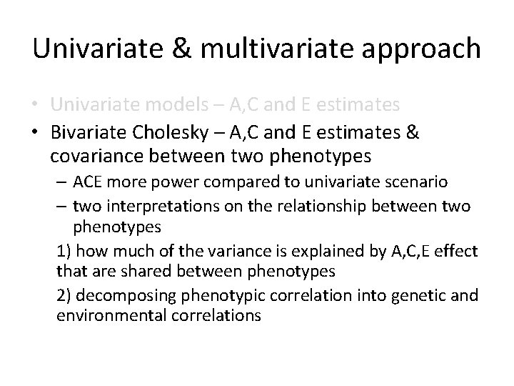
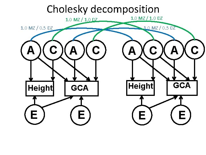
Univariate & multivariate approach • Univariate models – A, C and E estimates • Bivariate Cholesky – A, C and E estimates & covariance between two phenotypes – ACE more power compared to univariate scenario – two interpretations on the relationship between two phenotypes 1) how much of the variance is explained by A, C, E effect that are shared between phenotypes 2) decomposing phenotypic correlation into genetic and environmental correlations

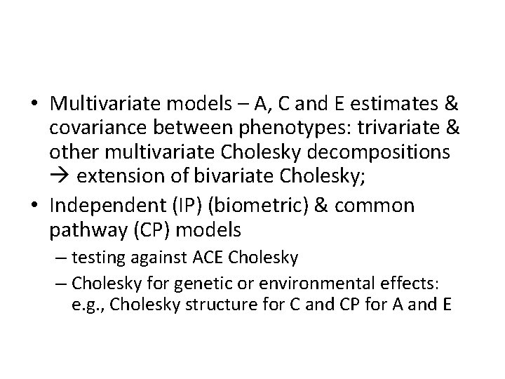
• Multivariate models – A, C and E estimates & covariance between phenotypes: trivariate & other multivariate Cholesky decompositions extension of bivariate Cholesky; • Independent (IP) (biometric) & common pathway (CP) models – testing against ACE Cholesky – Cholesky for genetic or environmental effects: e. g. , Cholesky structure for C and CP for A and E

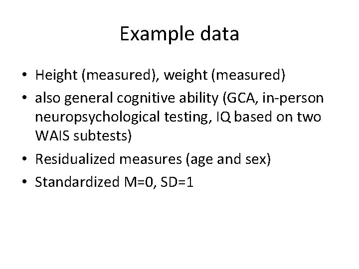
Example data • Height (measured), weight (measured) • also general cognitive ability (GCA, in-person neuropsychological testing, IQ based on two WAIS subtests) • Residualized measures (age and sex) • Standardized M=0, SD=1

Bivariate Vars <- c(’var 1', ’var 2') nv <- 2 # number of variables ntv <- nv*2 # number of total variables sel. Vars <- paste(Vars, c(rep(1, nv), rep(2, nv)), sep="") path. A <- mx. Matrix( type="Lower", nrow=nv, ncol=nv, free=TRUE, values= ? , lbound=? , ubound=? name="a" ) path. C <- mx. Matrix( type="Lower", nrow=nv, ncol=nv, free=TRUE, values= ? , lbound=? , ubound=? name=”c" ) path. E <- mx. Matrix( type="Lower", nrow=nv, ncol=nv, free=TRUE, values= ? , lbound=? , ubound=? name=”c" )

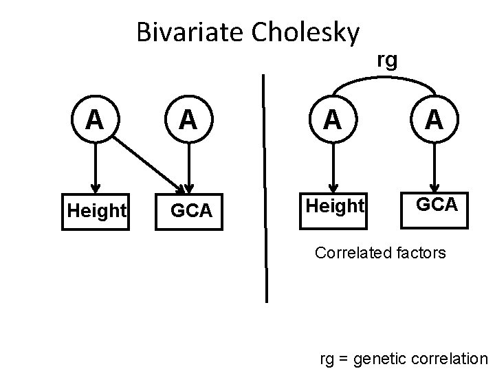
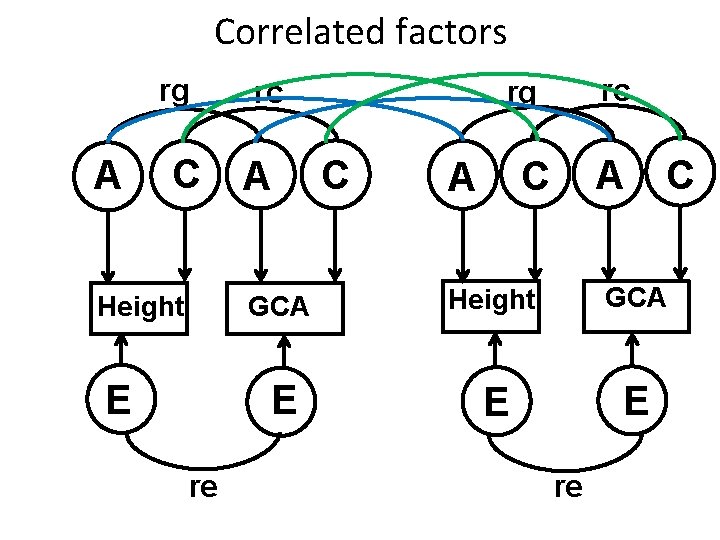
Bivariate Cholesky rg A A Height GCA Correlated factors rg = genetic correlation

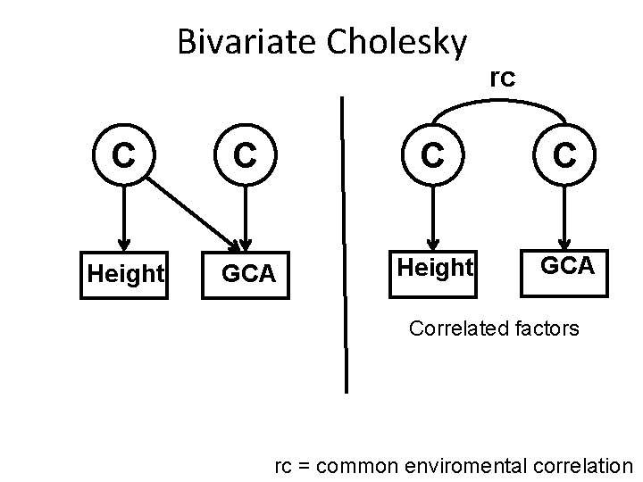
Bivariate Cholesky rc C C Height GCA Correlated factors rc = common enviromental correlation

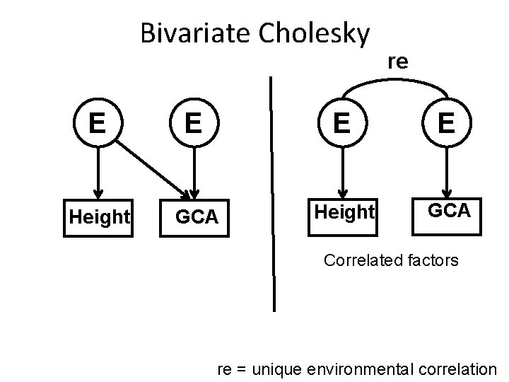
Bivariate Cholesky re E E Height GCA Correlated factors re = unique environmental correlation

Cholesky decomposition 1. 0 MZ / 1. 0 DZ 1. 0 MZ / 0. 5 DZ A C Height E 1. 0 MZ / 0. 5 DZ A C C A A C GCA Height GCA E E E

Correlated factors rg A C Height E re A rc rg rc C A C GCA Height GCA E E E re

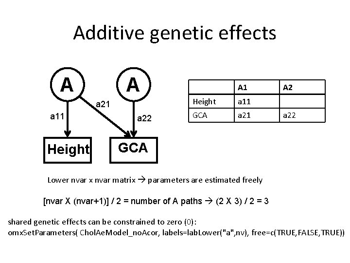
Additive genetic effects A A a 21 a 11 Height a 22 A 1 Height a 11 GCA a 21 A 2 a 22 GCA Lower nvar x nvar matrix parameters are estimated freely [nvar X (nvar+1)] / 2 = number of A paths (2 X 3) / 2 = 3 shared genetic effects can be constrained to zero (0): omx. Set. Parameters( Chol. Ae. Model_no. Acor, labels=lab. Lower("a", nv), free=c(TRUE, FALSE, TRUE))

Additive genetic effects C C c 21 c 11 Height c 22 C 1 Height c 11 GCA c 21 C 2 c 22 GCA Lower nvar x nvar matrix parameters are estimated freely [nvar X (nvar+1)] / 2 = number of C paths (2 X 3) / 2 = 3 shared common environmental effects can be constrained to zero (0): omx. Set. Parameters( Chol. Ae. Model_no. Ccor, labels=lab. Lower(”c", nv), free=c(TRUE, FALSE, TRUE))

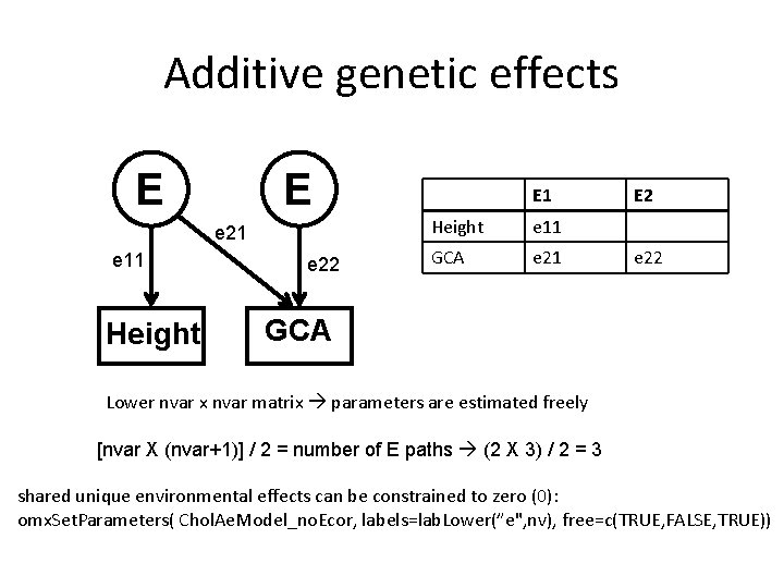
Additive genetic effects E E e 21 e 11 Height e 22 E 1 Height e 11 GCA e 21 E 2 e 22 GCA Lower nvar x nvar matrix parameters are estimated freely [nvar X (nvar+1)] / 2 = number of E paths (2 X 3) / 2 = 3 shared unique environmental effects can be constrained to zero (0): omx. Set. Parameters( Chol. Ae. Model_no. Ecor, labels=lab. Lower(”e", nv), free=c(TRUE, FALSE, TRUE))

Number of parameters Bivariate [nvar X (nvar+1)] / 2 = number of A paths (2 X 3) / 2 = 3 [nvar X (nvar+1)] / 2 = number of C paths (2 X 3) / 2 = 3 [nvar X (nvar+1)] / 2 = number of E paths (2 X 3) / 2 = 3 means = 2 number of parameters = 11 Number of parameters in AE-AE cholesky ? Number of parameters in AE-AE cholesky where rg = 0 ?

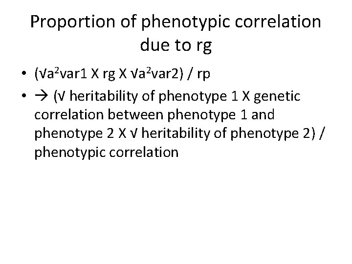
Proportion of phenotypic correlation due to rg • (√a 2 var 1 X rg X √a 2 var 2) / rp • (√ heritability of phenotype 1 X genetic correlation between phenotype 1 and phenotype 2 X √ heritability of phenotype 2) / phenotypic correlation

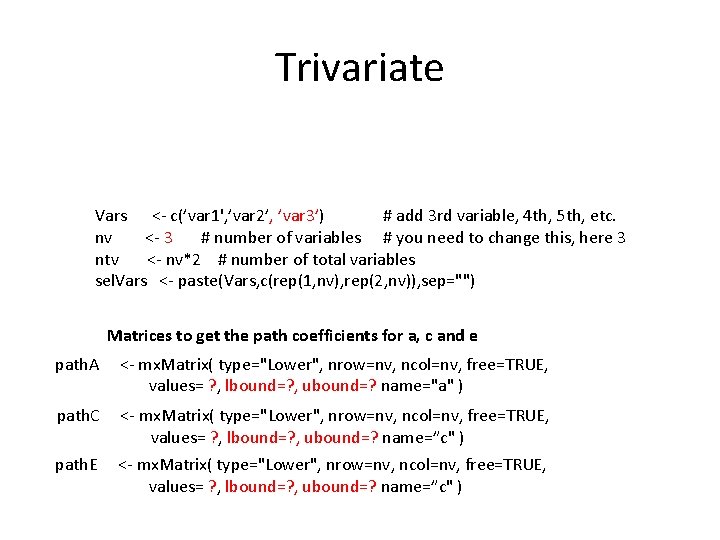
Trivariate Vars <- c(’var 1', ’var 2’, ’var 3’) # add 3 rd variable, 4 th, 5 th, etc. nv <- 3 # number of variables # you need to change this, here 3 ntv <- nv*2 # number of total variables sel. Vars <- paste(Vars, c(rep(1, nv), rep(2, nv)), sep="") Matrices to get the path coefficients for a, c and e path. A <- mx. Matrix( type="Lower", nrow=nv, ncol=nv, free=TRUE, values= ? , lbound=? , ubound=? name="a" ) path. C <- mx. Matrix( type="Lower", nrow=nv, ncol=nv, free=TRUE, values= ? , lbound=? , ubound=? name=”c" ) path. E <- mx. Matrix( type="Lower", nrow=nv, ncol=nv, free=TRUE, values= ? , lbound=? , ubound=? name=”c" )

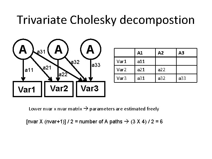
Trivariate Cholesky decompostion A a 11 Var 1 A A a 31 a 32 a 21 a 33 a 22 Var 2 A 1 A 2 Var 1 a 11 Var 2 a 21 a 22 Var 3 a 31 a 32 Var 3 Lower nvar x nvar matrix parameters are estimated freely [nvar X (nvar+1)] / 2 = number of A paths (3 X 4) / 2 = 6 A 3 a 33

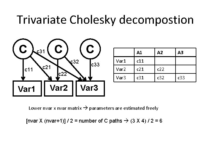
Trivariate Cholesky decompostion C c 11 Var 1 C C c 31 c 32 c 21 c 33 c 22 Var 2 A 1 A 2 Var 1 c 11 Var 2 c 21 c 22 Var 3 c 31 c 32 Var 3 Lower nvar x nvar matrix parameters are estimated freely [nvar X (nvar+1)] / 2 = number of C paths (3 X 4) / 2 = 6 A 3 c 33

Trivariate Cholesky decompostion E e 11 Var 1 E E e 31 e 32 e 21 e 33 e 22 Var 2 A 1 A 2 Var 1 e 11 Var 2 e 21 e 22 Var 3 e 31 e 32 Var 3 Lower nvar x nvar matrix parameters are estimated freely [nvar X (nvar+1)] / 2 = number of E paths (3 X 4) / 2 = 6 A 3 e 33

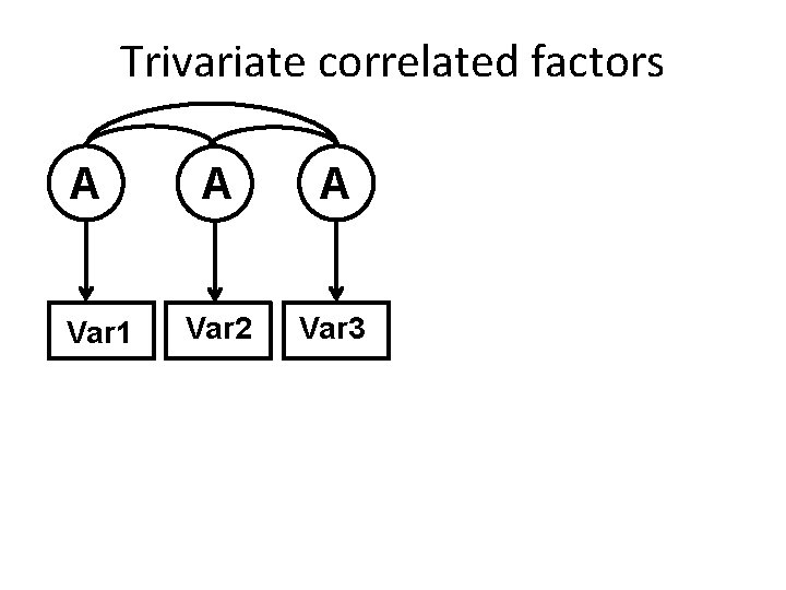
Trivariate correlated factors A Var 1 A A Var 2 Var 3

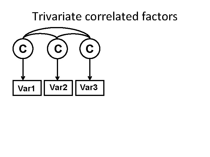
Trivariate correlated factors C Var 1 C C Var 2 Var 3

Trivariate correlated factors E Var 1 E E Var 2 Var 3

Number of parameters Trivariate [nvar X (nvar+1)] / 2 = number of A paths [nvar X (nvar+1)] / 2 = number of C paths [nvar X (nvar+1)] / 2 = number of E paths means number of parameters = ?

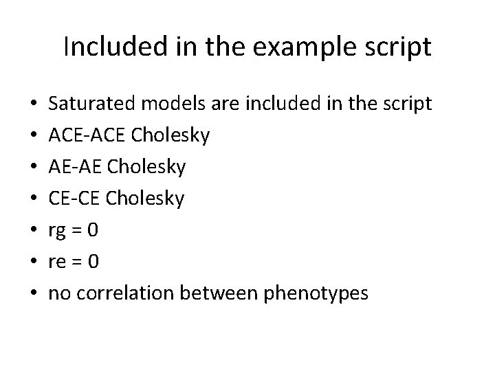
Included in the example script • • Saturated models are included in the script ACE-ACE Cholesky AE-AE Cholesky CE-CE Cholesky rg = 0 re = 0 no correlation between phenotypes

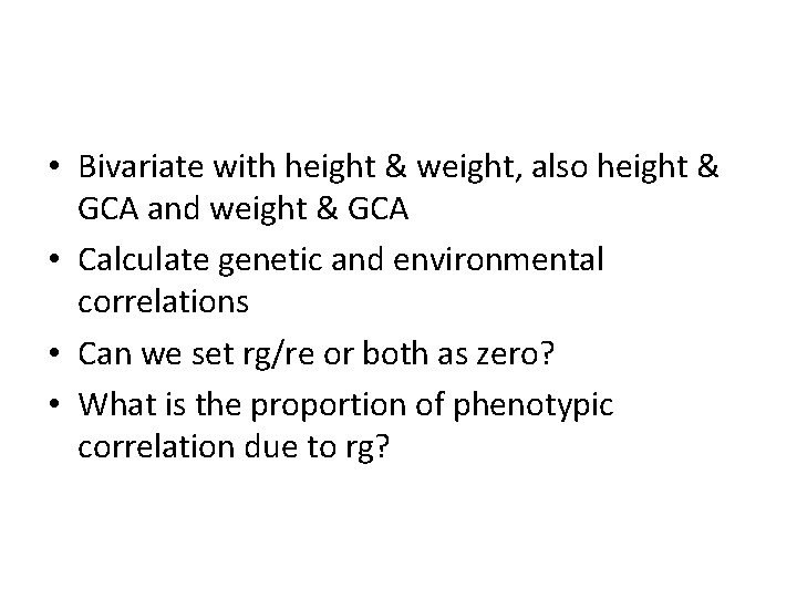
• Bivariate with height & weight, also height & GCA and weight & GCA • Calculate genetic and environmental correlations • Can we set rg/re or both as zero? • What is the proportion of phenotypic correlation due to rg?

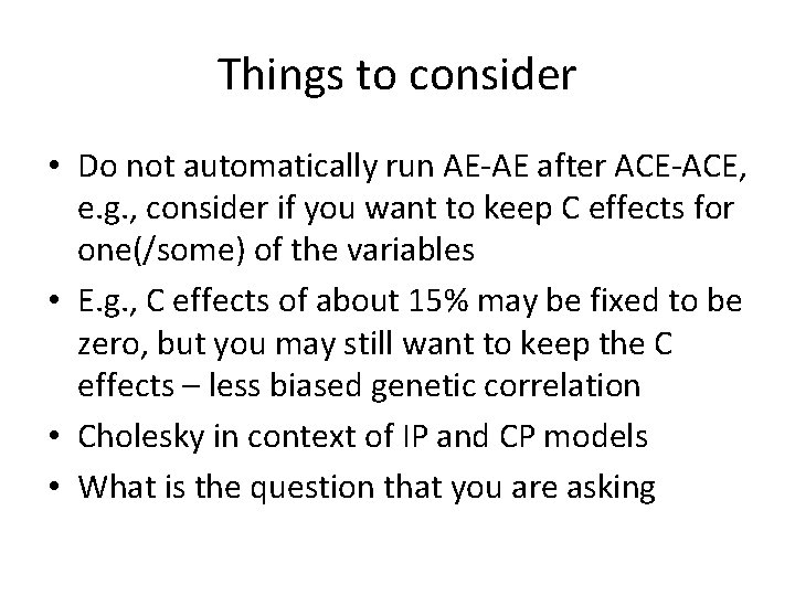
Things to consider • Do not automatically run AE-AE after ACE-ACE, e. g. , consider if you want to keep C effects for one(/some) of the variables • E. g. , C effects of about 15% may be fixed to be zero, but you may still want to keep the C effects – less biased genetic correlation • Cholesky in context of IP and CP models • What is the question that you are asking

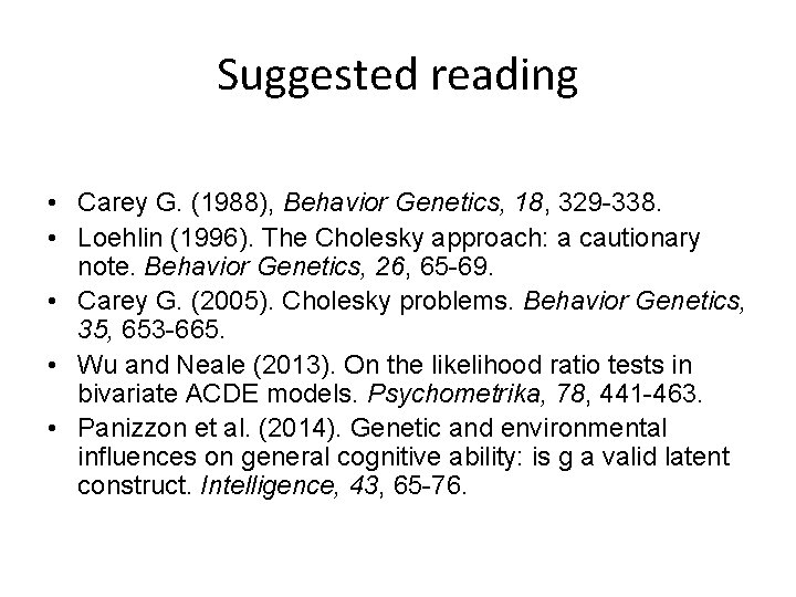
Suggested reading • Carey G. (1988), Behavior Genetics, 18, 329 -338. • Loehlin (1996). The Cholesky approach: a cautionary note. Behavior Genetics, 26, 65 -69. • Carey G. (2005). Cholesky problems. Behavior Genetics, 35, 653 -665. • Wu and Neale (2013). On the likelihood ratio tests in bivariate ACDE models. Psychometrika, 78, 441 -463. • Panizzon et al. (2014). Genetic and environmental influences on general cognitive ability: is g a valid latent construct. Intelligence, 43, 65 -76.

Resources including presentations • International Twin workshop, every March, Institute for behavioral genetics, University of Boulder Colorado • QIMR, Workshop, Sarah Medland